US8006239B2 - Program analysis using symbolic ranges - Google Patents

Program analysis using symbolic ranges Download PDF

Info

Publication number
US8006239B2
US8006239B2 US12/015,126 US1512608A US8006239B2 US 8006239 B2 US8006239 B2 US 8006239B2 US 1512608 A US1512608 A US 1512608A US 8006239 B2 US8006239 B2 US 8006239B2
Authority
US
United States
Prior art keywords
src
computer
implemented method
program
srcs
Prior art date
Legal status (The legal status is an assumption and is not a legal conclusion. Google has not performed a legal analysis and makes no representation as to the accuracy of the status listed.)
Expired - Fee Related, expires
Application number
US12/015,126
Other versions
US20080172653A1 (en
Inventor
Sriram SANKARANARAYANAN
Aarti Gupta
Franjo Ivancic
Ilya SHLYAKHTER
Current Assignee (The listed assignees may be inaccurate. Google has not performed a legal analysis and makes no representation or warranty as to the accuracy of the list.)
NEC Corp
Original Assignee
NEC Laboratories America Inc
Priority date (The priority date is an assumption and is not a legal conclusion. Google has not performed a legal analysis and makes no representation as to the accuracy of the date listed.)
Filing date
Publication date
Application filed by NEC Laboratories America Inc filed Critical NEC Laboratories America Inc
Priority to US12/015,126 priority Critical patent/US8006239B2/en
Assigned to NEC LABORATORIES AMERICA, INC. reassignment NEC LABORATORIES AMERICA, INC. ASSIGNMENT OF ASSIGNORS INTEREST (SEE DOCUMENT FOR DETAILS). Assignors: SHLYAKHTER, ILYA, GUPTA, AARTI, IVANCIC, FRANJO, SANKARANARAYANAN, SRIRAM
Publication of US20080172653A1 publication Critical patent/US20080172653A1/en
Application granted granted Critical
Publication of US8006239B2 publication Critical patent/US8006239B2/en
Assigned to NEC CORPORATION reassignment NEC CORPORATION ASSIGNMENT OF ASSIGNORS INTEREST (SEE DOCUMENT FOR DETAILS). Assignors: NEC LABORATORIES AMERICA, INC.
Expired - Fee Related legal-status Critical Current
Adjusted expiration legal-status Critical

Links

Images

Classifications

    • GPHYSICS
    • G06COMPUTING; CALCULATING OR COUNTING
    • G06FELECTRIC DIGITAL DATA PROCESSING
    • G06F11/00Error detection; Error correction; Monitoring
    • G06F11/36Preventing errors by testing or debugging software
    • G06F11/3604Software analysis for verifying properties of programs

Definitions

  • This invention relates generally to the of program analysis and in particular to program analysis techniques that derives symbolic bounds on variable values used in computer programs.
  • Interval analysis is but one technique used to determine static lower and upper bounds on values of computer program variables. While these determined interval bounds are useful—especially for inferring invariants to prove buffer overflow checks—they nevertheless are inadequate as invariants due to a lack of relational information among the variables.
  • Interval Ranges see, e.g., Patrick Cousot & Radhia Cousot, “Static Determination of Dynamic Properties of Program”, Proceedings of the Second International Symposium on Programming , pp. 106-130, 1976
  • Polyhedra see, e.g., Patrick Cousot & Nicholas Halbwachs, “Automatic Discovery of linear restraints among the variables of a program”, ACM Principles of Programming Languages , pp 84-97, 1979
  • Octagons see Antoine Mine, PhD Thesis, autoimmune Normale Superiure, 2005
  • abstract domains that provide representations and algorithms sufficient to carry out abstract interpretation. They are targeted towards buffer overflow detection by computing variable ranges but can be applicable to other applications as well.
  • SRC Symbolic Range Constraints
  • FIG. 1(A) is a program excerpt for a motivating example of the present invention
  • FIG. 1(B) is a sliced control follow graph for the example of FIG. 1(A) ;
  • FIG. 1(C) is an interval analysis for the example of FIG. 1(A) ;
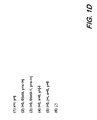
  • FIG. 1(D) is a symbolic range analysis for the example of FIG. 1(A) ;
  • FIG. 2(A) depicts a 2D hexagon while FIGS. 2(B)-2(E) are a series of four possible abstractions of that 2D hexagon;
  • FIG. 3(A)-3(C) show three situations encountered during abstraction.
  • FIG. 1(A) For our purposes herein, we illustrate symbolic ranges for invariant computation using a motivating example presented in FIG. 1(A) . With reference to that figure, and assuming that the analysis starts at the function foo, we analyze whether the assertion at the end of the function holds.
  • FIG. 1(B) shows a control flow graph for this example after program slicing.
  • FIG. 1(C) shows an interval analysis computation for this example. In this example, interval analysis is not powerful enough to conclude that the assertion can never be violated.
  • R represent the reals and R + , the set of extended reals (R ⁇ ⁇ ).
  • ⁇ right arrow over (x) ⁇ denote a vector of n>0 real-valued variables.
  • the i th component of the vector ⁇ right arrow over (x) ⁇ is written x i .
  • A, B, C to denote matrices.
  • x 1 x 2 . . . x n we fix a variable ordering given by x 1 x 2 . . . x n , with the index i of a variable x i being synonymous with its rank in this ordering.
  • a linear expression is of the form e: ⁇ right arrow over (c) ⁇ T ⁇ right arrow over (x) ⁇ +d where ⁇ right arrow over (c) ⁇ is a vector of coefficients over the reals, while d ⁇ R + is the constant coefficient.
  • a linear expression of the form c T ⁇ right arrow over (x) ⁇ is identical to ⁇ right arrow over (0) ⁇ T ⁇ right arrow over (x) ⁇ .
  • the expression 2x 1 + ⁇ is identical to 0x 1 + ⁇ .
  • a linear constraint is a conjunction of finitely many linear inequalities ⁇ : ⁇ i e i ⁇ 0.
  • e i 1 c i ⁇ e - x i .
  • the sign denotes the reversal of the direction of the inequality if c i ⁇ 0.
  • a symbolic range constraint (SRC) is of the form ⁇ : l i ⁇ x i ⁇ u i where for each i ⁇ [l,n], the linear expressions l i ,u i are made up of variables in the set ⁇ x i+1 , . . . ,x n ⁇ . In particular, l n ,u n are constants. The linear assertions false and true are also assumed to be srcs.
  • ⁇ :x 2 +4 ⁇ x 1 ⁇ 2x 3 +x 2 +4 ⁇ x 3 ⁇ x 2 ⁇ x 3 +4 ⁇ x 3 ⁇ 0 is a SRC.
  • the variable ordering is x 1 x 2 x 3 .
  • the bound for x l involves ⁇ x 2 ,x 3 ⁇ , x 2 involves ⁇ x 3 ⁇ and x 3 has constant bounds.
  • Implied constraints & normalization Given a symbolic range l i ⁇ x i ⁇ u i , its implied inequality is l i ⁇ u i . Note that the implied inequality l i ⁇ u i only involves variables x i+1 , . . . ,x n .
  • the SRC ⁇ from Example 1 is not normalized.
  • the implied constraint 0 ⁇ 2x 3 derived from the range x 2 +4 ⁇ x 1 ⁇ 2x 3 +x 2 +4 is not implied by ⁇ [2] .
  • the equivalent SRC ⁇ ′ is normalized: ⁇ ′: x 2 +4 ⁇ x 1 ⁇ 2 x 3 +x 2 +4 ⁇ x 3 ⁇ x 2 ⁇ x 3 +4 0 ⁇ x 3 ⁇ 0
  • the SRC ⁇ :x 2 ⁇ x 3 ⁇ x 1 ⁇ 1 0 ⁇ x 2 ⁇ 2 0 ⁇ x 3 ⁇ 2 forms a counter-example.
  • the projection of ⁇ on the ⁇ x 2 ,x 3 ⁇ is a five sided polygon, whereas any SRC in 2D is a trapezium.
  • each intermediate expression e i involves only the variables in ⁇ x i+1 , . . . ,x n ⁇ . Specifically, e n ⁇ .
  • optimization for SRCs can also be solved by efficient algorithms such as SIMPLEX or interior point techniques.
  • SIMPLEX or interior point techniques.
  • weak optimization since (a) it out-performs LP solvers, (b) is less dependent on floating point arithmetic, and (c) allows us to draw sound inferences wherever required.
  • well-known examples such as Klee-Minty cubes and Goldfarb cubes that exhibit worst case behavior for SIMPLEX algorithms happen to be SRCs. It is unclear if such SRCs will arise in practical verification problems.
  • Abstraction converts arbitrary first-order formulae to symbolic ranges. In practice, programs we analyze are first linearized. Therefore, abstraction needs to be defined only on polyhedra. Abstraction is used as a primitive operation that organizes arbitrary linear constraints into the form of SRCs.
  • be a polyhedron represented as a conjunction of linear inequalities e i ⁇ 0.
  • SRC ⁇ : ⁇ ( ⁇ ) such that ⁇ ⁇ .
  • this SRC abstraction ⁇ ( ⁇ ) may not be uniquely defined.
  • FIG. 2(A)-FIG . 2 (D) there is shown a series of four possible SRC abstractions for a hexagon in 2 dimensions that are all semantically incomparable.
  • An Abstraction of a given polyhedron ⁇ is performed by sequentially inserting the inequalities of ⁇ into a target SRC, starting initially with the SRC true.
  • the result is an SRC ⁇ ( ⁇ ).
  • FIG. 3 there is shown a series of three cases FIG. 3(A)-FIG . 3 (C) encountered during abstraction.
  • FIG. 3(A) b j u j the bound x j ⁇ u j entails x j ⁇ b j , therefore we need not replace u j .
  • FIG. 3(B) the bound x j ⁇ u j entails x j ⁇ b j , therefore we need not replace u j .
  • FIG. 3(B) and u j is replaced.
  • neither bound entails the other. We call this a conflict.
  • Metric Heuristic When employing a metric heuristic, we first choose the bound that minimizes the volume of the resulting SRC, or alternatively, the distance from a reference set.
  • LexOrder Heuristic When employing a LexOrder heuristic, we choose syntactically according to lexicographic order.
  • a fixed heuristic involves always choosing to retain the original bound u j , or replace it with b j .
  • the abstraction algorithm is parameterized by the conflict resolution heuristic.
  • Our implementation uses the interval heuristic to resolve conflicts and the lexicographic order to break ties. For example, we let ⁇ denote the abstraction function that uses some conflict resolution strategy.
  • ⁇ ( ⁇ ) is a SRC and ⁇ ⁇ ( ⁇ ).
  • a SRC ⁇ may fail to be normalized in the course of our analysis as a result of abstraction or other domain operations. Failure of normalization can itself be detected in O(n 3 ) time using weak optimization using the lemma below:
  • a SRC ⁇ is normalized iff for each bound l i ⁇ x i ⁇ u i , 0 ⁇ i ⁇ n, ⁇ [i+1] l i ⁇ u i . Note that the relation is sufficient to test normalization.
  • Top-down normalization Add constant offsets ⁇ j , ⁇ j >0 to bounds l j ,u j such that the resulting bounds l j ⁇ j ⁇ x j ⁇ u j + ⁇ j are normalized.
  • ⁇ j , ⁇ j may be computed by recursively normalizing ⁇ [j+1] and then using weak optimization. As a corollary of Lemma 3, the top-down normalization technique always normalizes.
  • Lemma 4 Let ⁇ be an SRC and ⁇ 1 , ⁇ 2 be the results of applying bottom-up and top-down techniques, respectively to ⁇ . It follows that ⁇ ⁇ 1 and ⁇ ⁇ 2 . However, ⁇ ⁇ 1 does not always hold.
  • the best possible join ⁇ 1 ⁇ 2 for SRCs ⁇ 1 , ⁇ 2 can be defined as the abstraction of the polyhedral convex hull ⁇ 1 , ⁇ 2 .
  • convex hull computations are expensive, even for SRCs.
  • Projection is an important primitive for implementing the transfer function across assignments and modeling scope in inter-procedural analysis.
  • the “best” projection is, in general, the abstraction of the projection carried out over polyhedra.
  • polyhedral projection is an exponential time operation in the worst case.
  • Definition 5 A variable z occurring in the RHS of a bound x j b j has positive polarity if b j is a lower bound and z has a positive coefficient, or b j is an upper bound and z has a negative coefficient. The variable has negative polarity otherwise. Variable z with positive polarity in a constraint is written z ⁇ , and negative polarity as z ⁇ (see Example 7).
  • Direct projection Consider the projection of x j from SRC ⁇ . Let l j ⁇ x j ⁇ u j denote the bounds for the variable x j in ⁇ . For an occurrence of x j in a bound inequality of the form x i b i : ⁇ right arrow over (c) ⁇ T ⁇ right arrow over (x) ⁇ +d (note i ⁇ j by triangulation), we replace x j in this expression by one of l j ,u j based on the polarity replacement rule: occurrences of x j + are replaced by the lower bound l j , and x j ⁇ are by u j . Finally, x j and its bounds are removed from the constraint. Direct projection can be computed in time O(n 2 ).
  • ⁇ ′ be the result of a simple projection of x j from ⁇ . It follows that ⁇ ′ is an SRC and ( ⁇ x j ) ⁇ ⁇ ′. Direct projection of z from ⁇ :z + ⁇ x ⁇ z ⁇ +1 z + ⁇ 2 ⁇ y ⁇ z ⁇ +3 ⁇ z ⁇ 5, replaces z + with ⁇ and z ⁇ with 5 at each occurrence, yielding ⁇ ′: ⁇ x ⁇ 6 ⁇ y ⁇ 8.
  • direct projection can be improved by using a simple modification of Fourier-Motzkin elimination technique.
  • a matching pair for the variable x j consists of two occurrences of variable x j with opposite polarities in bounds x i ⁇ j x j + +e i and x k ⁇ j x j ⁇ +e k with i ⁇ k.
  • the matching pairs for the SRC ⁇ from Example 7 are:
  • the matching pair z + ⁇ x and y ⁇ z ⁇ +3 can be used to rewrite the former constraint as: y ⁇ 3 ⁇ x.
  • the other matching pair can be used to rewrite the upper bound of x to x ⁇ y+2.
  • An indirect projection of the constraint in Example 7, using matching pairs yields the result y ⁇ 3 ⁇ x ⁇ y+ 3 ⁇ y ⁇ 8.
  • Matching pairs can be used to improve over direct projection, especially when the existing bounds for the variables to be projected may lead to too coarse an over-approximation. They are sound and preserve the triangular structure.
  • substitution x j e involves the replacement of every occurrence of x j in the constraint by e.
  • the result of carrying out the replacements is not a SRC.
  • the abstraction algorithm can be used to reconstruct a SRC as ⁇ ′: ⁇ ( ⁇ [x e]).
  • a better widening operator is obtained by first replacing each occurrence of x j ⁇ (x j occurring with negative polarity) by a matching pair before replacing u j .
  • Lower bounds such as x j ⁇ l j are handled symmetrically.
  • Lemma 7 The SRC widening ⁇ R satisfies (a) ⁇ 1 , ⁇ 2 ⁇ 1 ⁇ R ⁇ 2 ; (b) any ascending chain eventually converges (even if is used to detect convergence), i.e., for any sequence ⁇ 1 , . . . , ⁇ n , . . . , the widened sequence ⁇ 1 , . . . , satisfies ⁇ N+1 ⁇ N , for some N>0.
  • the SRC narrowing is similar to the interval narrowing. Let ⁇ 2 ⁇ 1 .
  • the narrowing ⁇ 1 ⁇ r ⁇ 2 is given by replacing every ⁇ bound in ⁇ 1 by the corresponding bound in ⁇ 2 .
  • Equalities While equalities can be captured in the SRC domain itself, it is beneficial to compute the equality constraints separately.
  • A is a n ⁇ n matrix.
  • variable ordering allows us to share information between the two domains. For instance, ⁇ bounds for the SRC component can be replaced with bounds inferred from the equality constraints during the course of the analysis.
  • the equality invariants can also be used to delay widening. Following the polyhedral widening operator of Bagnara et al., we do not apply widening if the equality part has decreased in rank during the iteration.
  • variable ordering used in the analysis has a considerable impact on its precision.
  • the ideal choice of a variable ordering requires us to assign the higher indices to variables which are likely to be unbounded, or have constant bounds.
  • a variable x is defined in terms of y in the program flow, it is more natural to express the bounds of x in terms of y than the other way around.
  • variables used as loop counters, or array indices are assigned lower indices than loop bounds or those that track array/pointer lengths.
  • variables used as arguments to functions have higher indices than local variables inside functions.
  • Variables of a similar type are ordered using data dependencies.
  • a dataflow analysis is used to track dependencies among a variable. If the dependency information between two variables is always uni-directional we use this information to determine a variable ordering. Finally, variables which cannot be otherwise ordered in a principled way are ordered randomly.
  • the tool constructs a CFG representation from the program, which is simplified using program slicing, constant propagation, and optionally by interval analysis.
  • a linearization abstraction converts operations such as multiplication and integer division into non-deterministic choices.
  • Arrays and pointers are modeled by their allocated sizes while array contents are abstracted away.
  • Pointer aliasing is modeled soundly using a flow insensitive alias analysis.
  • Variable clustering The analysis model size is reduced by creating small clusters of related variables. For each cluster, statements that involve variables not belonging to the current cluster are abstracted away. The analysis is performed on these abstractions. A property is considered proved only if it can be proved in each context by some cluster abstraction. Clusters are detected heuristically by a backward traversal of the CFG, collecting the variables that occur in the same expressions or conditions. The backward traversal is stopped as soon as the number of variables in a cluster first exceeds 20 variables for our experiments. The number of clusters ranges from a few hundreds to nearly 2000 clusters.
  • the fixpoint computation is performed by means of an upward iteration using widening to converge to some fixed point followed by a downward iteration using narrowing to improve the fixed point until no more improvements are possible.
  • the iteration strategy used is semi-naive. At each step, we minimize the number of applications of post conditions by keeping track of nodes whose abstract state changed in the previous iteration.
  • the narrowing phase is cut off after a fixed number of iteration to avoid potential non termination.
  • Table 1(A) and 1(B) summarizes the results on these examples.
  • Table 1(A) shows the total running times and the number of properties established. The properties proved by the domains are compared pairwise. The pairwise comparison summarizes the number of properties that each domain could (not) prove as compared to other domains.
  • the SRC domain comes out slightly ahead in terms of proofs, while remaining competitive in terms of time. An analysis of the failed proofs revealed that roughly 25 are due to actual bugs (mostly unintentional) in the programs, while the remaining were mostly due to modeling limitations.
  • Root functions are chosen based on their position in the global call graph. Each analysis run first simplifies the model using slicing, constant folding and interval analysis.
  • Table 3 shows each of these functions along with the number of properties sliced away as a result of all the front-end simplifications. Also note that a large fraction of the properties can be handled simply by using interval analysis and constant folding. Slicing the CFG to remove these properties triggers a large reduction in the CFG size.
  • Table 4 compares the performance of the SRC domain with the octagon and polyhedral domains on the CFG simplified by slicing, constant folding and intervals.
  • the interval domain captures many of the easy properties including the common case of static arrays accessed in loops with known bounds. While the SRC and octagon domains can complete on all the examples even in the absence of such simplifications, running interval analysis as a pre-processing step nevertheless lets us focus on those properties for which domains such as octagons, SRC and polyhedra are really needed. In many situations, the domains produce a similar bottom line. Nevertheless, there are cases where SRCs capture proofs missed by octagons and polyhedra.
  • the SRC domain takes roughly 2.5 ⁇ more time than the octagon domain.
  • the polyhedral domain proves much fewer properties than both octagons and SRCs in this experiment, while requiring significantly more time.
  • iteration strategy used especially the fast onset of widening and the narrowing cutoff for polyhedra may account for the discrepancy.
  • increasing either parameter only serve to slow the analysis down further.
  • precise widening operators along with techniques such as lookahed widening, landmark-based widening or widening with acceleration can compensate for the lack of a good polyhedral narrowing.

Abstract

A computer implemented method for generating a representation of relationships between variables in a program employing Symbolic Range Constraints (SRCs) wherein the SRCs are of the form φ:^i=1 nli≦xi≦ui where for each i ε[l,n], the linear expressions li,ui are made up of variables in the set{xi+1, . . . ,xn} and wherein the SRCs comprise linear, convex, and triangulated constraints for a given variable order.

Description

CROSS REFERENCE TO RELATED APPLICATIONS
This application claims the benefit of U.S. Provisional Application No. 60/885,028 filed Jan. 16, 2007.
FIELD OF THE INVENTION
This invention relates generally to the of program analysis and in particular to program analysis techniques that derives symbolic bounds on variable values used in computer programs.
BACKGROUND OF THE INVENTION
Interval analysis is but one technique used to determine static lower and upper bounds on values of computer program variables. While these determined interval bounds are useful—especially for inferring invariants to prove buffer overflow checks—they nevertheless are inadequate as invariants due to a lack of relational information among the variables.
Abstract Interpretation (see Patrick Cousot & Radhia Cousot, ACM Principles of Programming Languages, 1977) is a framework that allows us to analyze programs to infer useful information such as intervals for variables. An abstract interpretation over a program requires us to define some basic components in a mathematically well-defined way to carry out program analysis automatically. By the way of further background, commercial as well as freely available tools such as F-Soft(NEC Laboratories America), Astree(Airbus Inc.), PolySpace(Mathworks Inc.) and CodeSonar(GrammaTech Inc.) implement the generic abstract interpretation algorithm. To instantiate such frameworks, we need to arrive at suitable representation (abstract domain objects) and algorithms to perform the following mathematical operations on the representation: (a) Join, (b)Intersection, (c)Transfer Function, (d) Projection, (e) Widening, (f) Narrowing and (g) Inclusion check.
Any mathematically sound (see e.g., Patrick Cousot & Radhia Cousot, “Abstract Interpretation: A unified lattice model for static analysis of programs by construction or approximation of fixpoints”, ACM Principles of Programming Languages, pp. 238-252, 1977.) definition of the representation accompanied by algorithms to carry out operations (a-f) described above constitute a mathematically sound abstract domain. Such domains can be used as black-boxes by the frameworks mentioned above to perform useful program analysis tasks oriented towards program verification, optimization and other applications of this framework.
Interval Ranges (see, e.g., Patrick Cousot & Radhia Cousot, “Static Determination of Dynamic Properties of Program”, Proceedings of the Second International Symposium on Programming, pp. 106-130, 1976), Polyhedra (see, e.g., Patrick Cousot & Nicholas Halbwachs, “Automatic Discovery of linear restraints among the variables of a program”, ACM Principles of Programming Languages, pp 84-97, 1979) and Octagons (see Antoine Mine, PhD Thesis, Ecole Normale Superiure, 2005) are examples of abstract domains that provide representations and algorithms sufficient to carry out abstract interpretation. They are targeted towards buffer overflow detection by computing variable ranges but can be applicable to other applications as well.
SUMMARY OF THE INVENTION
An advance is made in the art according to the principles of the present invention directed to a computer implemented technique for deriving symbolic bounds on computer program variable values using abstract interpretation.
We provide a new representation: Symbolic Range Constraints (SRC) and describe algorithms for operations join, intersection, transfer functions, widening, narrowing, projection and inclusion check to enable the implementation of an abstract interpretation scheme using SRCs.
BRIEF DESCRIPTION OF THE DRAWING
A more complete understanding of the present invention may be realized by reference to the accompanying drawings in which:
FIG. 1(A) is a program excerpt for a motivating example of the present invention;
FIG. 1(B) is a sliced control follow graph for the example of FIG. 1(A);
FIG. 1(C) is an interval analysis for the example of FIG. 1(A);
FIG. 1(D) is a symbolic range analysis for the example of FIG. 1(A);
FIG. 2(A) depicts a 2D hexagon while FIGS. 2(B)-2(E) are a series of four possible abstractions of that 2D hexagon;
FIG. 3(A)-3(C) show three situations encountered during abstraction.
DETAILED DESCRIPTION
The following merely illustrates the principles of the invention. It will thus be appreciated that those skilled in the art will be able to devise various arrangements which, although not explicitly described or shown herein, embody the principles of the invention and are included within its spirit and scope.
Furthermore, all examples and conditional language recited herein are principally intended expressly to be only for pedagogical purposes to aid the reader in understanding the principles of the invention and the concepts contributed by the inventor(s) to furthering the art, and are to be construed as being without limitation to such specifically recited examples and conditions.
Moreover, all statements herein reciting principles, aspects, and embodiments of the invention, as well as specific examples thereof, are intended to encompass both structural and functional equivalents thereof. Additionally, it is intended that such equivalents include both currently known equivalents as well as equivalents developed in the future, i.e., any elements developed that perform the same function, regardless of structure.
Thus, for example, the diagrams herein represent conceptual views of illustrative structures embodying the principles of the invention.
For our purposes herein, we illustrate symbolic ranges for invariant computation using a motivating example presented in FIG. 1(A). With reference to that figure, and assuming that the analysis starts at the function foo, we analyze whether the assertion at the end of the function holds. FIG. 1(B) shows a control flow graph for this example after program slicing. FIG. 1(C) shows an interval analysis computation for this example. In this example, interval analysis is not powerful enough to conclude that the assertion can never be violated.
1. A Motivating Example
Consider the analysis using symbolic ranges, for the variable ordering i,j, x, y (see FIG. 1(D)). Since symbolic ranges can represent the loop invariant y=x−i+j, the analysis discovers that for x=y=0 which implies that i=j at the point of the assertion. Note also that this assertion cannot be proved using octagons, since the loop invariant is not expressible in terms of octagonal relationships.
2. Symbolic Range Constraints
We now provide a description of the symbolic range constraints (SRCs) and the basic algorithms required to implement abstract interpretation schemes using SRCs. The description and examples provided in this section are at a level of detail sufficient for any practitioner skilled in the art of building program analyzers to effectively apply our invention.
Let R represent the reals and R+, the set of extended reals (R ∪ {±∞}). Let {right arrow over (x)} denote a vector of n>0 real-valued variables. The ith component of the vector {right arrow over (x)} is written xi. We use A, B, C to denote matrices. Throughout this section, we fix a variable ordering given by x1
Figure US08006239-20110823-P00001
x2
Figure US08006239-20110823-P00001
. . .
Figure US08006239-20110823-P00001
xn, with the index i of a variable xi being synonymous with its rank in this ordering.
A linear expression is of the form e:{right arrow over (c)}T{right arrow over (x)}+d where {right arrow over (c)} is a vector of coefficients over the reals, while d ε R+ is the constant coefficient. By convention, a linear expression of the form cT{right arrow over (x)}±∞ is identical to {right arrow over (0)}T{right arrow over (x)}±∞. For instance, the expression 2x1+∞ is identical to 0x1+∞. A linear inequality is of the form e
Figure US08006239-20110823-P00002
0, where
Figure US08006239-20110823-P00003
{≧,≦,=}. A linear constraint is a conjunction of finitely many linear inequalities φ:^iei≧0.
Given an inequality e≧0, where e is not a constant, its lead variable xi is the least index i s.t. ci≠0. We may write such an inequality in the bounded form
Figure US08006239-20110823-P00004
, where xi is the lead variable and
e i = 1 c i e - x i .
The sign
Figure US08006239-20110823-P00005
denotes the reversal of the direction of the inequality if ci<0.
As an example, consider the inequality 2x2+3x5+1≦0. Its lead variable is X2 and bounded form is
x 2 - 3 2 x 5 - 1 2 .
We reuse the
Figure US08006239-20110823-P00006
relation to denote entailment among linear constraints in the first order theory of linear arithmetic.
Definition 3—Symbolic Range Constraint: A symbolic range constraint (SRC) is of the form φ:
Figure US08006239-20110823-P00007
li≦xi≦ui where for each i ε [l,n], the linear expressions li,ui are made up of variables in the set {xi+1, . . . ,xn}. In particular, ln,un are constants. The linear assertions false and true are also assumed to be srcs.
The absence of a bound for xj is modeled by setting the bound to ±∞. Given an SRC φ:
Figure US08006239-20110823-P00008
lj≦xj≦uj, let φ[i] denote the assertion
Figure US08006239-20110823-P00009
lj≦xj≦uj.
EXAMPLE 1
φ:x2+4≦x1≦2x3+x2+4
Figure US08006239-20110823-P00010
−x3≦x2≦x3+4
Figure US08006239-20110823-P00010
−∞≦x3≦0 is a SRC. The variable ordering is x1
Figure US08006239-20110823-P00001
x2
Figure US08006239-20110823-P00001
x3. The bound for xl involves {x2,x3}, x2 involves {x3} and x3 has constant bounds.
Implied constraints & normalization. Given a symbolic range li≦xi≦ui, its implied inequality is li≦ui. Note that the implied inequality li≦ui only involves variables xi+1, . . . ,xn.
Definition 4—Normalization: A SRC is normalized iff for each variable bound li≦xi≦ui, φ[i+1]
Figure US08006239-20110823-P00006
li≦ui. By convention, the empty and universal SRC are normalized.
EXAMPLE 2
The SRC φ from Example 1 is not normalized. The implied constraint 0≦2x3 derived from the range x2+4≦x1≦2x3+x2+4 is not implied by φ[2]. The equivalent SRC φ′ is normalized:
φ′:x 2+4≦x 1≦2x 3 +x 2+4
Figure US08006239-20110823-P00010
x 3 ≦x 2 ≦x 3+4
Figure US08006239-20110823-P00010
0≦x 3≦0
Unfortunately, not every SRC has a normal equivalent. The SRC ψ:x2−x3≦x1≦1
Figure US08006239-20110823-P00010
0≦x2≦2
Figure US08006239-20110823-P00010
0≦x3≦2 forms a counter-example. The projection of ψ on the {x2,x3} is a five sided polygon, whereas any SRC in 2D is a trapezium.
Weak optimization algorithms: Optimization is used repeatedly as a primitive for other domain operations including abstraction, join and intersection. Consider the optimization instance min.(e:{right arrow over (c)}T{right arrow over (x)}+d)s.t.φ. Let φ be a satisfiable SRC with bound lj≦xj≦uj for index 0≦j<n. We let
Figure US08006239-20110823-C00001

denote the replacement of xj in e by lj (lower bound in φ) if its coefficient in e is positive, or uj otherwise.
Formally,
e = { e - c j x j + c j l j , c j 0 e - c j x j + c j u j , c j < 0
The canonical sequence, given by
Figure US08006239-20110823-C00002

replaces variables in the ascending order of their indices. The canonical sequence, denoted in short by
Figure US08006239-20110823-C00003

is unique and yields a unique result. The following lemma follows from the triaangulation of SRCs.
Lemma 1: For the canonical sequence
Figure US08006239-20110823-C00004

each intermediate expression ei involves only the variables in {xi+1, . . . ,xn}. Specifically, en ε
Figure US08006239-20110823-P00011
.
EXAMPLE 3
Consider the SRC φ′ defined in Example 2 and the expression: e: −3x1+2x2+8x3. This yields the sequence:
Figure US08006239-20110823-C00005

It follows that en under-approximates the minima of the optimization problem, and if φ is normalized, weak optimization computes the exact minima; the same result as any other LP solver.
Theorem 1—Weak Optimization Theorem: Given a constraint φ and the sequence eφ en, φ
Figure US08006239-20110823-P00006
e≧en. Furthermore, if φ is normalized then en=min es.t.φ.
Weak optimization requires O(n) rewriting steps, each in turn involving arithmetic over expressions of size O(n). Therefore, the complexity of weak optimization for a SRC with n constraints is O(n2).
EXAMPLE 4
From Theorem 1, it may be determined that −16 is the exact minimum in Example 3. Consider the equivalent constraint φ from Example 1. The same objective minimizes to −∞ (unbounded) if performed w.r.t. φ.
Optimization provides an inference mechanism: given d=min es.t.φ, we infer φ
Figure US08006239-20110823-P00012
e≧d. By Theorem 1, an inference using weak optimization is always sound. It is also complete, if the constraint φ is also normalized. Given SRC φ, we write φ
Figure US08006239-20110823-P00013
e≧0 to denote inference of e≧0 from φ by weak optimization. Similarly, φ
Figure US08006239-20110823-P00013
^iei≧0 iff (∀i)φ
Figure US08006239-20110823-P00013
ei≧0.
Optimization for SRCs can also be solved by efficient algorithms such as SIMPLEX or interior point techniques. We refer to such techniques as strong optimization techniques. In practice, however, we prefer weak optimization since (a) it out-performs LP solvers, (b) is less dependent on floating point arithmetic, and (c) allows us to draw sound inferences wherever required. As a curiosity, we also note that well-known examples such as Klee-Minty cubes and Goldfarb cubes that exhibit worst case behavior for SIMPLEX algorithms happen to be SRCs. It is unclear if such SRCs will arise in practical verification problems.
For our purposes herein, we assume optimization is always performed using weak optimization. Nevertheless, any call to weak optimization can be substituted by a call to strong optimization. Experimental results provide further justification for this choice.
We also use optimization to compare expressions wrt a given SRC φ. We write e1
Figure US08006239-20110823-P00014
e2 iff φ
Figure US08006239-20110823-P00013
e1≧e2. Expressions are equivalent, written e1φe2, if φ
Figure US08006239-20110823-P00006
e1=e2, and incomparable, denoted ee2, if neither inequality holds.
Abstraction. The abstraction function converts arbitrary first-order formulae to symbolic ranges. In practice, programs we analyze are first linearized. Therefore, abstraction needs to be defined only on polyhedra. Abstraction is used as a primitive operation that organizes arbitrary linear constraints into the form of SRCs.
Let ψ be a polyhedron represented as a conjunction of linear inequalities
Figure US08006239-20110823-P00015
ei≧0. We seek a SRC φ:α(ψ) such that ψ
Figure US08006239-20110823-P00006
φ. Unfortunately, this SRC abstraction α(ψ) may not be uniquely defined. Turning now to FIG. 2(A)-FIG. 2(D), there is shown a series of four possible SRC abstractions for a hexagon in 2 dimensions that are all semantically incomparable.
An Abstraction of a given polyhedron ψ is performed by sequentially inserting the inequalities of ψ into a target SRC, starting initially with the SRC true. The result is an SRC α(ψ).
Inequality Insertion. Let φ be a SRC and ej≧0 be an inequality. As a primitive we consider the problem of deriving an abstraction α(φ
Figure US08006239-20110823-P00010
ej≧0). We consider the case wherein xj≦bj is the bounded form of ej. The case where the bounded form is xj≧bj is handled symmetrically. Also, let lj≦xj≦uj be the existing bounds for xj in φ.
Turning our attention now to FIG. 3, there is shown a series of three cases FIG. 3(A)-FIG. 3(C) encountered during abstraction. Using expression comparison, we distinguish three cases, FIG. 3(A) bj
Figure US08006239-20110823-P00016
uj, FIG. 3(B) uj
Figure US08006239-20110823-P00017
bj and FIG. 3(C) u [j+1] bj. For the case shown in FIG. 3(A), the bound xj≦uj entails xj≦bj, therefore we need not replace uj. The reverse holds for the case shown in FIG. 3(B), and uj is replaced. However, for case shown in FIG. 3(C), neither bound entails the other. We call this a conflict.
A conflict forces us to choose between two bounds uj,bj where neither is semantically stronger than the other. Conflicts are due to the lack of a unique SRC abstraction. We handle conflicts using conflict resolution heuristics provided by the user. We now describe a few of the possible heuristics
Interval Heuristic: When employing an interval heuristic, we consider the worst case interval bound on xj resulting from either choice of bounds. Let c=max bjs.t.φ[j+1] and similarly, d=max ujs.t.φ[j+1]. If c<d, we replace uj by bj, and retain uj otherwise. A geometric interpretation of such is shown diagrammatically in FIG. 3(C).
Metric Heuristic: When employing a metric heuristic, we first choose the bound that minimizes the volume of the resulting SRC, or alternatively, the distance from a reference set.
LexOrder Heuristic: When employing a LexOrder heuristic, we choose syntactically according to lexicographic order.
Fixed Heuristic: A fixed heuristic involves always choosing to retain the original bound uj, or replace it with bj.
The result of abstraction is not guaranteed to be normalized. If there are no conflicts in the abstraction process then semantic equivalence of the SRC to the original polyhedron follows. In summary, the abstraction algorithm is parameterized by the conflict resolution heuristic. Our implementation uses the interval heuristic to resolve conflicts and the lexicographic order to break ties. For example, we let α denote the abstraction function that uses some conflict resolution strategy.
Lemma 2. For a constraint ψ, α(ψ) is a SRC and ψ
Figure US08006239-20110823-P00006
α(ψ).
Each inequality insertion requires us to solve finitely many optimization problems. Weak optimization requires time O(n2). Therefore, the SRC abstraction a polyhedron with m inequalities can be computed in time O(n2m).
4. Domain Operations
With these details in place, we may now discuss the implementation of various operations required for static analysis over SRCs.
Forced normalization. A SRC φ may fail to be normalized in the course of our analysis as a result of abstraction or other domain operations. Failure of normalization can itself be detected in O(n3) time using weak optimization using the lemma below:
Lemma 3. A SRC φ is normalized iff for each bound li≦xi≦ui, 0≦i<n, φ[i+1]
Figure US08006239-20110823-P00013
li≦ui. Note that the
Figure US08006239-20110823-P00013
relation is sufficient to test normalization.
Bottom-up normalization: In general, a SRC that is not normalized may not have a normal equivalent. However, it is frequently the case that normalization may be achieved by simply propagating missing information from lower order indices up to the higher order indices. We consider each bound lj≦xj≦uj, for j=n−1, . . . ,1, and insert the implied inequality lj≦uj into φ[j+1] using the abstraction procedure described previously. This process does not always produce a normalized constraint. However, the procedure itself is useful since it can sometimes replace missing bounds for variables by using a bound implied by the remaining constraints.
EXAMPLE 5
Recall the SRC φ from Example 3. The implied inequality x2+4(≦x1)≦2x3+x2+4 simplifies to x3≧0. When inserted, this yields the normalized SRC φ′ from Example 2.
Even though bottom-up normalization is not always guaranteed to succeed, it generally improves the result of the weak optimization algorithm. We therefore employ it after other domain operations as a pre-normalization step.
Top-down normalization: Add constant offsets αjj>0 to bounds lj,uj such that the resulting bounds lj−αj≦xj≦ujj are normalized. In practice, αjj may be computed by recursively normalizing φ[j+1] and then using weak optimization. As a corollary of Lemma 3, the top-down normalization technique always normalizes.
Lemma 4: Let φ be an SRC and φ12 be the results of applying bottom-up and top-down techniques, respectively to φ. It follows that φ
Figure US08006239-20110823-P00006
φ1 and φ
Figure US08006239-20110823-P00013
φ2. However, φ
Figure US08006239-20110823-P00013
φ1 does not always hold.
Following other numerical domains, we note that normalization should never be forced after a widening operation to ensure termination.
Intersection & join. Given two SRCs φ1
Figure US08006239-20110823-P00010
φ2 their intersection can be performed by using the abstraction procedure, i.e., φ1
Figure US08006239-20110823-P00018
φ2=α(φ1
Figure US08006239-20110823-P00010
φ2). In general, the best possible join φ1
Figure US08006239-20110823-P00019
φ2 for SRCs φ12 can be defined as the abstraction of the polyhedral convex hull φ12. However, convex hull computations are expensive, even for SRCs.
We now describe a direct generalization of the interval join used for value ranges. Let lj≦xj≦uj be a bound in φ1 (similar analysis is used for bounds in φ2). Consider the following optimization problems:
c j 1=min.x j −l j s.t.φ 2 , d j 1=max.x j −u j s.t.φ 2.
Note that φ2
Figure US08006239-20110823-P00006
lj+cj 1≦xj≦uj+dj 1, while φ1
Figure US08006239-20110823-P00006
lj+0≦xj≦uj+0. As a result, (φ1
Figure US08006239-20110823-P00019
φ2)
Figure US08006239-20110823-P00006
lj+min(cj 1,0)≦xj≦uj+max(0,dj 1). We call such a constraint the relaxation of xj in φ1. Let φ12 be the result of relaxing each bound in φ1 wrt φ2. Similarly, let φ21 be obtained by relaxing each bound in φ2 wrt φ1. We define the range join as φ1
Figure US08006239-20110823-P00020
φ212
Figure US08006239-20110823-P00018
φ21.
Lemma 5. Given any SRC φ12, φi
Figure US08006239-20110823-P00013
φ1
Figure US08006239-20110823-P00020
φ2, i=1,2. Also, φ1
Figure US08006239-20110823-P00018
φ2
Figure US08006239-20110823-P00006
φi. However, this containment may not be provable using
Figure US08006239-20110823-P00013
.
Relaxing each constraint requires O(n) optimization, each requiring O(n2) time. Finally, abstraction itself requires O(n3) time. As a result join can be achieved in time O(n3).
EXAMPLE 6
Consider the SRCs φ12 shown below:
φ 1 : { x 2 x 1 2 x 2 + 4 x 3 x 2 5 - 4 x 3 4 } φ 2 : { - x 1 x 2 0 x 2 x 3 + 1 0 x 3 2 }
The relaxed constraints are given by
φ 12 : { - x 1 2 x 2 + 4 x 3 - 2 x 2 5 - 4 x 3 4 } φ 21 : { - x 1 x 2 + 9 - 4 x 2 x 3 + 9 - 4 x 3 4 }
The join is computed by intersecting these constraints:
φ:−∞≦x 1≦2x 2+4
Figure US08006239-20110823-P00010
x 3−2≦x 2≦5
Figure US08006239-20110823-P00010
−4≦x 3≦4.
Projection. Projection is an important primitive for implementing the transfer function across assignments and modeling scope in inter-procedural analysis. The “best” projection is, in general, the abstraction of the projection carried out over polyhedra. However, like convex hull, polyhedral projection is an exponential time operation in the worst case.
Definition 5—Polarity: A variable z occurring in the RHS of a bound xj
Figure US08006239-20110823-P00002
bj has positive polarity if bj is a lower bound and z has a positive coefficient, or bj is an upper bound and z has a negative coefficient. The variable has negative polarity otherwise. Variable z with positive polarity in a constraint is written z, and negative polarity as z (see Example 7).
Direct projection: Consider the projection of xj from SRC φ. Let lj≦xj≦uj denote the bounds for the variable xj in φ. For an occurrence of xj in a bound inequality of the form xi
Figure US08006239-20110823-P00002
bi:{right arrow over (c)}T{right arrow over (x)}+d (note i<j by triangulation), we replace xj in this expression by one of lj,uj based on the polarity replacement rule: occurrences of xj + are replaced by the lower bound lj, and xj are by uj. Finally, xj and its bounds are removed from the constraint. Direct projection can be computed in time O(n2).
Lemma 6: Let φ′ be the result of a simple projection of xj from φ. It follows that φ′ is an SRC and (∃xj
Figure US08006239-20110823-P00006
φ′. Direct projection of z from φ:z+≦x≦z+1
Figure US08006239-20110823-P00010
z+−2≦y≦z+3
Figure US08006239-20110823-P00010
−∞≦z≦5, replaces z+ with −∞ and z with 5 at each occurrence, yielding φ′:−∞≦x≦6
Figure US08006239-20110823-P00010
−∞≦y≦8.
Indirect projection. Advantageously, direct projection can be improved by using a simple modification of Fourier-Motzkin elimination technique. A matching pair for the variable xj consists of two occurrences of variable xj with opposite polarities in bounds xi
Figure US08006239-20110823-P00002
αjxj ++ei and xk
Figure US08006239-20110823-P00002
αjxj +ek with i≠k. The matching pairs for the SRC φ from Example 7 are:
Figure US08006239-20110823-C00006
There are two matching pairs for the variable z shown using arrows. The matching pair z+≦x and y≦z+3 can be used to rewrite the former constraint as: y−3≦x. Similarly the other matching pair can be used to rewrite the upper bound of x to x≦y+2. An indirect projection of the constraint in Example 7, using matching pairs yields the result
y−3≦x≦y+3
Figure US08006239-20110823-P00010
−∞≦y≦8.
Matching pairs can be used to improve over direct projection, especially when the existing bounds for the variables to be projected may lead to too coarse an over-approximation. They are sound and preserve the triangular structure.
Substitution. The substitution xj
Figure US08006239-20110823-P00021
e involves the replacement of every occurrence of xj in the constraint by e. In general, the result of carrying out the replacements is not a SRC. However, the abstraction algorithm can be used to reconstruct a SRC as φ′:α(φ[x
Figure US08006239-20110823-P00021
e]).
Transfer function. Consider a SRC φ and an assignment xj:=e, where e≡{right arrow over (c)}T{right arrow over (x)}+d. The assignment is invertible if cj≠0, on the other hand the assignment is non-invertible or destructive if cj=0. An invertible assignment can be handled using a substitution
ψ : φ [ x j 1 c j ( x j - ( e - c j x j ) ) ] .
A destructive update is handled by first using the projection algorithm to compute φ′:∃xjφ and then computing the intersection ψ:α(φ′
Figure US08006239-20110823-P00010
xj=e) using the abstraction algorithm.
Widening. An instance of widening consists of two SRCs φ12 such that φ1
Figure US08006239-20110823-P00006
φ2. Using widening, we simply drop each constraint in φ1 that is not entailed by φ2. Let xj≦uj be an upper bound in φ1. We first compute cj=max.(xj−uj)s.t.φ2. If cj>0 then φ2
Figure US08006239-20110823-P00022
Wxj≦uj. Therefore, we need to drop the constraint. This may be done by replacing the bound uj with ∞. A better widening operator is obtained by first replacing each occurrence of xj (xj occurring with negative polarity) by a matching pair before replacing uj. Lower bounds such as xj≧lj are handled symmetrically.
Lemma 7 The SRC widening ∇R satisfies (a) φ12
Figure US08006239-20110823-P00013
φ1Rφ2; (b) any ascending chain eventually converges (even if
Figure US08006239-20110823-P00013
is used to detect convergence), i.e., for any sequence ψ1, . . . ,ψn, . . . , the widened sequence φ1, . . . , satisfies φN+1
Figure US08006239-20110823-P00013
φN, for some N>0.
Narrowing. The SRC narrowing is similar to the interval narrowing. Let φ2
Figure US08006239-20110823-P00006
φ1. The narrowing φ1Δrφ2 is given by replacing every ±∞ bound in φ1 by the corresponding bound in φ2.
Lemma 8. For any SRCs φ1 and φ2, s.t. φ2
Figure US08006239-20110823-P00006
φ1, φ1Δrφ2
Figure US08006239-20110823-P00006
φ1. Furthermore, the narrowing iteration for SRC domain converges.
Equalities. While equalities can be captured in the SRC domain itself, it is beneficial to compute the equality constraints separately. An equality constraint can be stored as A{right arrow over (x)}+{right arrow over (b)}=0 where A is a n×n matrix. In practice, we store A in its triangulated form assuming some ordering on the variables. Therefore, it is possible to construct the product domain of SRC and linear equalities wherein both domains share the same variable ordering. The equality part is propagated using Karr's analysis.
Using the same variable ordering allows us to share information between the two domains. For instance, ±∞ bounds for the SRC component can be replaced with bounds inferred from the equality constraints during the course of the analysis. The equality invariants can also be used to delay widening. Following the polyhedral widening operator of Bagnara et al., we do not apply widening if the equality part has decreased in rank during the iteration.
Variable Ordering
We now consider the choice of the variable ordering. The variable ordering used in the analysis has a considerable impact on its precision. The ideal choice of a variable ordering requires us to assign the higher indices to variables which are likely to be unbounded, or have constant bounds. Secondly, if a variable x is defined in terms of y in the program flow, it is more natural to express the bounds of x in terms of y than the other way around. We therefore consider two factors in choosing a variable ordering: (a) ordering based on variable type or its purpose in the code; and (b) ordering based on variable dependencies.
The determination of the “type” or “purpose” of a variable is made using syntactic templates. For instance, variables used as loop counters, or array indices are assigned lower indices than loop bounds or those that track array/pointer lengths. Similarly, variables used as arguments to functions have higher indices than local variables inside functions. These variables are identified in the front end during CFG construction using a simple variable dependency analysis.
Variables of a similar type are ordered using data dependencies. A dataflow analysis is used to track dependencies among a variable. If the dependency information between two variables is always uni-directional we use this information to determine a variable ordering. Finally, variables which cannot be otherwise ordered in a principled way are ordered randomly.
5. Exemplary Implementation
We have implemented an exemplary analysis tool to prove array accesses safe as part of an ongoing. Our analyzer is targeted towards proving numerous runtime safety properties of C programs including array and pointer access checks. The analyzer is context sensitive, by using call strings to track contexts. While recursive functions cannot be handled directly, they may be abstracted by unrolling to some fixed length and handling the remaining calls context insensitively. Our abstract interpreter supports a combination of different numerical domains, including constant folding, interval, octagon, polyhedron and SRC domains. For our experiments, we used off-the-shelf implementations of the octagon abstract domain library, and the Parma Polyhedron Library. Each library was used with the same abstract interpreter to carry out the program analysis.
The tool constructs a CFG representation from the program, which is simplified using program slicing, constant propagation, and optionally by interval analysis. A linearization abstraction converts operations such as multiplication and integer division into non-deterministic choices. Arrays and pointers are modeled by their allocated sizes while array contents are abstracted away. Pointer aliasing is modeled soundly using a flow insensitive alias analysis.
Variable clustering. The analysis model size is reduced by creating small clusters of related variables. For each cluster, statements that involve variables not belonging to the current cluster are abstracted away. The analysis is performed on these abstractions. A property is considered proved only if it can be proved in each context by some cluster abstraction. Clusters are detected heuristically by a backward traversal of the CFG, collecting the variables that occur in the same expressions or conditions. The backward traversal is stopped as soon as the number of variables in a cluster first exceeds 20 variables for our experiments. The number of clusters ranges from a few hundreds to nearly 2000 clusters.
Iteration Strategy. The fixpoint computation is performed by means of an upward iteration using widening to converge to some fixed point followed by a downward iteration using narrowing to improve the fixed point until no more improvements are possible. To improve the initial fixed point, the onset of widening is delayed by a fixed number of iterations (2 iterations for our experiments). The iteration strategy used is semi-naive. At each step, we minimize the number of applications of post conditions by keeping track of nodes whose abstract state changed in the previous iteration. In the case of the polyhedral domain, the narrowing phase is cut off after a fixed number of iteration to avoid potential non termination.
6. Experiments
Our experiments involved the verification of C programs for runtime errors such as buffer overflows, null pointer accesses, and string library usage checks. The domains are compared simply based on their ability to prove properties.
Small Benchmarks. We first compare the domains on a collection of small example programs. These programs are written in the C language, and range from 20-400 lines of code. The examples typically consist of statically or dynamically allocated arrays accessed inside loops using aliased pointers, and passed as parameters to string/standard library functions.
Table 1(A) and 1(B) summarizes the results on these examples. Table 1(A) shows the total running times and the number of properties established. The properties proved by the domains are compared pairwise. The pairwise comparison summarizes the number of properties that each domain could (not) prove as compared to other domains. In general, the SRC domain comes out slightly ahead in terms of proofs, while remaining competitive in terms of time. An analysis of the failed proofs revealed that roughly 25 are due to actual bugs (mostly unintentional) in the programs, while the remaining were mostly due to modeling limitations.
Comparison of Implementation Choices. Our implementation of SRCs requires heuristics for optimization, variable ordering and conflict resolution while abstracting. Table 2 compares the proofs and running times for some alternative strategies for these operations. Each experiment in the table changes one option at a time, leaving the others unchanged. The choices we made for these strategies perform better than the more ad-hoc strategies used in these experiments. In particular, the difference is most pronounced when the variable ordering used is exactly the reverse of that suggested by our heuristic.
Network Controller Study. We studied the performance of our analyzer on a commercial network controller implementation. The analysis is started at different root functions assuming an unknown calling environment. Root functions are chosen based on their position in the global call graph. Each analysis run first simplifies the model using slicing, constant folding and interval analysis.
Table 3 shows each of these functions along with the number of properties sliced away as a result of all the front-end simplifications. Also note that a large fraction of the properties can be handled simply by using interval analysis and constant folding. Slicing the CFG to remove these properties triggers a large reduction in the CFG size.
Table 4 compares the performance of the SRC domain with the octagon and polyhedral domains on the CFG simplified by slicing, constant folding and intervals. The interval domain captures many of the easy properties including the common case of static arrays accessed in loops with known bounds. While the SRC and octagon domains can complete on all the examples even in the absence of such simplifications, running interval analysis as a pre-processing step nevertheless lets us focus on those properties for which domains such as octagons, SRC and polyhedra are really needed. In many situations, the domains produce a similar bottom line. Nevertheless, there are cases where SRCs capture proofs missed by octagons and polyhedra. The SRC domain takes roughly 2.5× more time than the octagon domain. On the other hand, the polyhedral domain proves much fewer properties than both octagons and SRCs in this experiment, while requiring significantly more time. We believe that the iteration strategy used, especially the fast onset of widening and the narrowing cutoff for polyhedra may account for the discrepancy. On the other hand, increasing either parameter only serve to slow the analysis down further. In general, precise widening operators along with techniques such as lookahed widening, landmark-based widening or widening with acceleration can compensate for the lack of a good polyhedral narrowing.
7. Conclusion
At this point, while we have discussed and described the invention using some specific examples, our teachings are not so limited. In particular, those skilled in the art will have recognized that we have described a technique employing an abstract domain using symbolic ranges that advantageously captures many properties that are missed by other domains such as octagons and intervals. Our technique does not incur the large time complexity of the polyhedral domain. Accordingly, we expect to use the SRC domain in conjunction with intervals, octagons and polyhedra to prove more properties while incurring a reasonable time overhead. Additionally, another interesting possibility is to allow for a conjunction of many SRC constraints, each using a different variable ordering. Apart from checking overflows, the SRC domain may also be useful for analyzing the numerical stability of floating point loops. The constraint handling techniques presented are therefore directly applied to practical tools such as ARCHER and ESP. Accordingly, the invention should be only limited by the scope of the claims attached hereto

Claims (13)

1. A computer-implemented method for generating a representation of relationships between variables in a program comprising the steps of:
automatically generating a set of Symbolic Range Constraints (SRCs) for the variables, wherein said SRCs are of the form φ:Λi=1 nli≦xi≦ui where for each i ε[l,n], the linear expressions li, ui are made up of variables in the set {xi+1, . . . , xn}, and wherein said SRCs comprise linear, convex, and triangulated constraints for a given variable order; and
providing said generated set of SRCs to a user.
2. The computer-implemented method of claim 1 employing a JOIN operation on SRC representations.
3. The computer-implemented method of claim 1 employing a MEET operation on SRC representations.
4. The computer-implemented method of claim 1 employing a transfer function of SRC representations with respect to a program statement.
5. The computer-implemented method of claim 1 employing a WIDENING operation on SRC representations.
6. The computer-implemented method of claim 1 employing a NARROWING operation on SRC representations.
7. The computer-implemented method of claim 1 further comprising the step of checking for inclusion of SRC representations.
8. The computer-implemented method of claim 1 which determines the correctness of the program by checking a safety property.
9. The computer-implemented method of claim 1 which determines the correctness of a program by detecting buffer overflow conditions.
10. The computer-implemented method of claim 1 which determines the correctness of a program by detecting null pointer dereferences.
11. The computer-implemented method of claim 1 which, used in an optimizing compiler, optimizes the program for size/performance.
12. The computer-implemented method of claim 1 which, used in a static analyzer, performs a program analysis.
13. The computer-implemented method of claim 1 which, used in a model checker, performs verification of the program.
US12/015,126 2007-01-16 2008-01-16 Program analysis using symbolic ranges Expired - Fee Related US8006239B2 (en)

Priority Applications (1)

Application Number Priority Date Filing Date Title
US12/015,126 US8006239B2 (en) 2007-01-16 2008-01-16 Program analysis using symbolic ranges

Applications Claiming Priority (2)

Application Number Priority Date Filing Date Title
US88502807P 2007-01-16 2007-01-16
US12/015,126 US8006239B2 (en) 2007-01-16 2008-01-16 Program analysis using symbolic ranges

Publications (2)

Publication Number Publication Date
US20080172653A1 US20080172653A1 (en) 2008-07-17
US8006239B2 true US8006239B2 (en) 2011-08-23

Family

ID=39618740

Family Applications (1)

Application Number Title Priority Date Filing Date
US12/015,126 Expired - Fee Related US8006239B2 (en) 2007-01-16 2008-01-16 Program analysis using symbolic ranges

Country Status (1)

Country Link
US (1) US8006239B2 (en)

Cited By (9)

* Cited by examiner, † Cited by third party
Publication number Priority date Publication date Assignee Title
US20080196017A1 (en) * 2005-08-30 2008-08-14 Tobias Ritzau Method and Software for Optimising the Positioning of Software Functions in a Memory
US20080301657A1 (en) * 2007-06-04 2008-12-04 Bowler Christopher E Method of diagnosing alias violations in memory access commands in source code
US20090249307A1 (en) * 2008-03-26 2009-10-01 Kabushiki Kaisha Toshiba Program analysis apparatus, program analysis method, and program storage medium
US20100162219A1 (en) * 2007-06-04 2010-06-24 International Business Machines Corporation Diagnosing Aliasing Violations in a Partial Program View
US20120185729A1 (en) * 2011-01-14 2012-07-19 Honeywell International Inc. Type and range propagation through data-flow models
US9183020B1 (en) 2014-11-10 2015-11-10 Xamarin Inc. Multi-sized data types for managed code
US9201637B1 (en) 2015-03-26 2015-12-01 Xamarin Inc. Managing generic objects across multiple runtime environments
US9213638B1 (en) 2015-03-24 2015-12-15 Xamarin Inc. Runtime memory management using multiple memory managers
US20170199731A1 (en) * 2015-11-02 2017-07-13 International Business Machines Corporation Method for defining alias sets

Families Citing this family (1)

* Cited by examiner, † Cited by third party
Publication number Priority date Publication date Assignee Title
US8266598B2 (en) * 2008-05-05 2012-09-11 Microsoft Corporation Bounding resource consumption using abstract interpretation

Citations (7)

* Cited by examiner, † Cited by third party
Publication number Priority date Publication date Assignee Title
US4642765A (en) * 1985-04-15 1987-02-10 International Business Machines Corporation Optimization of range checking
US6014723A (en) * 1996-01-24 2000-01-11 Sun Microsystems, Inc. Processor with accelerated array access bounds checking
US6343375B1 (en) * 1998-04-24 2002-01-29 International Business Machines Corporation Method for optimizing array bounds checks in programs
US6519765B1 (en) * 1998-07-10 2003-02-11 International Business Machines Corporation Method and apparatus for eliminating redundant array range checks in a compiler
US6665864B1 (en) * 1999-01-05 2003-12-16 International Business Machines Corporation Method and apparatus for generating code for array range check and method and apparatus for versioning
US7222337B2 (en) * 2001-05-31 2007-05-22 Sun Microsystems, Inc. System and method for range check elimination via iteration splitting in a dynamic compiler
US7260817B2 (en) * 1999-07-09 2007-08-21 International Business Machines Corporation Method using array range check information for generating versioning code before a loop for execution

Patent Citations (7)

* Cited by examiner, † Cited by third party
Publication number Priority date Publication date Assignee Title
US4642765A (en) * 1985-04-15 1987-02-10 International Business Machines Corporation Optimization of range checking
US6014723A (en) * 1996-01-24 2000-01-11 Sun Microsystems, Inc. Processor with accelerated array access bounds checking
US6343375B1 (en) * 1998-04-24 2002-01-29 International Business Machines Corporation Method for optimizing array bounds checks in programs
US6519765B1 (en) * 1998-07-10 2003-02-11 International Business Machines Corporation Method and apparatus for eliminating redundant array range checks in a compiler
US6665864B1 (en) * 1999-01-05 2003-12-16 International Business Machines Corporation Method and apparatus for generating code for array range check and method and apparatus for versioning
US7260817B2 (en) * 1999-07-09 2007-08-21 International Business Machines Corporation Method using array range check information for generating versioning code before a loop for execution
US7222337B2 (en) * 2001-05-31 2007-05-22 Sun Microsystems, Inc. System and method for range check elimination via iteration splitting in a dynamic compiler

Non-Patent Citations (8)

* Cited by examiner, † Cited by third party
Title
Blume et al., "Demand-Driven, Symbolic Range Propagation," 1995, p. 141-160. *
Blume et al., "Symbolic Range Propagation," 1995, IEEE, p. 357-363. *
Cousot et al., "Static Determination of Dynamic Properties of Programs," Apr. 1976, pp. 106-130. *
Markovskiy, Yury, "Range Analysis with Abstract Interpretation," Dec. 2002, p. 1-8. *
Rugina et al., "Symbolic Bounds Analysis of Pointers, Array Indices, and Accessed Memory Regions," Mar. 2005, ACM, p. 185-235. *
Su et al., "A Class of Polynomially Solvable Range Constraints for Interval Analysis withoutWidenings and Narrowings," 2004. *
Xie et al., "Archer: Using Symbolic, Pathsensitive Analysis to Detect Memory Access Errors," 2003, ACM. *
Zaks et al., "Range Analysis for Software Verification," 2006, p. 1-17. *

Cited By (17)

* Cited by examiner, † Cited by third party
Publication number Priority date Publication date Assignee Title
US8191055B2 (en) * 2005-08-30 2012-05-29 Sony Ericsson Mobile Communications Ab Method and software for optimising the positioning of software functions in a memory
US20080196017A1 (en) * 2005-08-30 2008-08-14 Tobias Ritzau Method and Software for Optimising the Positioning of Software Functions in a Memory
US8930927B2 (en) * 2007-06-04 2015-01-06 International Business Machines Corporation Diagnosing aliasing violations in a partial program view
US20080301657A1 (en) * 2007-06-04 2008-12-04 Bowler Christopher E Method of diagnosing alias violations in memory access commands in source code
US20100162219A1 (en) * 2007-06-04 2010-06-24 International Business Machines Corporation Diagnosing Aliasing Violations in a Partial Program View
US8839218B2 (en) 2007-06-04 2014-09-16 International Business Machines Corporation Diagnosing alias violations in memory access commands in source code
US20090249307A1 (en) * 2008-03-26 2009-10-01 Kabushiki Kaisha Toshiba Program analysis apparatus, program analysis method, and program storage medium
US8984488B2 (en) * 2011-01-14 2015-03-17 Honeywell International Inc. Type and range propagation through data-flow models
US20120185729A1 (en) * 2011-01-14 2012-07-19 Honeywell International Inc. Type and range propagation through data-flow models
US9183020B1 (en) 2014-11-10 2015-11-10 Xamarin Inc. Multi-sized data types for managed code
US9459847B2 (en) 2014-11-10 2016-10-04 Xamarin Inc. Multi-sized data types for managed code
US10061567B2 (en) 2014-11-10 2018-08-28 Microsoft Technology Licensing, Llc Multi-sized data types for managed code
US9213638B1 (en) 2015-03-24 2015-12-15 Xamarin Inc. Runtime memory management using multiple memory managers
US10657044B2 (en) 2015-03-24 2020-05-19 Xamarin Inc. Runtime memory management using multiple memory managers
US9201637B1 (en) 2015-03-26 2015-12-01 Xamarin Inc. Managing generic objects across multiple runtime environments
US20170199731A1 (en) * 2015-11-02 2017-07-13 International Business Machines Corporation Method for defining alias sets
US10223088B2 (en) * 2015-11-02 2019-03-05 International Business Machines Corporation Method for defining alias sets

Also Published As

Publication number Publication date
US20080172653A1 (en) 2008-07-17

Similar Documents

Publication Publication Date Title
US8006239B2 (en) Program analysis using symbolic ranges
D'silva et al. A survey of automated techniques for formal software verification
US8131768B2 (en) Symbolic program analysis using term rewriting and generalization
US7120902B2 (en) Method and apparatus for automatically inferring annotations
US8719802B2 (en) Interprocedural exception method
Tsitovich et al. Loop summarization and termination analysis
US20060248515A1 (en) Sound transaction-based reduction without cycle detection
US8719793B2 (en) Scope bounding with automated specification inference for scalable software model checking
US8589888B2 (en) Demand-driven analysis of pointers for software program analysis and debugging
Jacobs et al. Featherweight verifast
US7779382B2 (en) Model checking with bounded context switches
Cerny et al. Quantitative abstraction refinement
Vasconcelos Space cost analysis using sized types
Sankaranarayanan et al. Program analysis using symbolic ranges
Gulwani et al. A polynomial-time algorithm for global value numbering
Bouajjani et al. Lazy TSO reachability
Monat Static type and value analysis by abstract interpretation of Python programs with native C libraries
US7555418B1 (en) Procedure summaries for multithreaded software
US20110078511A1 (en) Precise thread-modular summarization of concurrent programs
De Angelis et al. Verifying array programs by transforming verification conditions
Tomb et al. Detecting inconsistencies via universal reachability analysis
Kyveli et al. Inclusion testing of Büchi automata based on well-quasiorders
Yu et al. Incremental predicate analysis for regression verification
Maurer Holmes: Binary analysis integration through datalog
Cuadrado et al. Deriving OCL optimization patterns from benchmarks

Legal Events

Date Code Title Description
AS Assignment

Owner name: NEC LABORATORIES AMERICA, INC., NEW JERSEY

Free format text: ASSIGNMENT OF ASSIGNORS INTEREST;ASSIGNORS:SANKARANARAYANAN, SRIRAM;GUPTA, AARTI;IVANCIC, FRANJO;AND OTHERS;REEL/FRAME:020629/0865;SIGNING DATES FROM 20080129 TO 20080306

Owner name: NEC LABORATORIES AMERICA, INC., NEW JERSEY

Free format text: ASSIGNMENT OF ASSIGNORS INTEREST;ASSIGNORS:SANKARANARAYANAN, SRIRAM;GUPTA, AARTI;IVANCIC, FRANJO;AND OTHERS;SIGNING DATES FROM 20080129 TO 20080306;REEL/FRAME:020629/0865

STCF Information on status: patent grant

Free format text: PATENTED CASE

AS Assignment

Owner name: NEC CORPORATION, JAPAN

Free format text: ASSIGNMENT OF ASSIGNORS INTEREST;ASSIGNOR:NEC LABORATORIES AMERICA, INC.;REEL/FRAME:027767/0918

Effective date: 20120224

FPAY Fee payment

Year of fee payment: 4

FEPP Fee payment procedure

Free format text: MAINTENANCE FEE REMINDER MAILED (ORIGINAL EVENT CODE: REM.); ENTITY STATUS OF PATENT OWNER: LARGE ENTITY

LAPS Lapse for failure to pay maintenance fees

Free format text: PATENT EXPIRED FOR FAILURE TO PAY MAINTENANCE FEES (ORIGINAL EVENT CODE: EXP.); ENTITY STATUS OF PATENT OWNER: LARGE ENTITY

STCH Information on status: patent discontinuation

Free format text: PATENT EXPIRED DUE TO NONPAYMENT OF MAINTENANCE FEES UNDER 37 CFR 1.362

FP Lapsed due to failure to pay maintenance fee

Effective date: 20190823