
DFSNet: A 3D Point Cloud Segmentation Network toward Trees Detection in an Orchard Scene

School of Electrical and Information Engineering, Jiangsu University, Zhenjiang 212000, China
*
Author to whom correspondence should be addressed.
Sensors 2024, 24(7), 2244; https://doi.org/10.3390/s24072244
Submission received: 4 March 2024
/
Revised: 29 March 2024
/
Accepted: 30 March 2024
/
Published: 31 March 2024
(This article belongs to the Special Issue Artificial Intelligence and Sensor Technologies in Agri-Food)
Abstract
:In order to guide orchard management robots to realize some tasks in orchard production such as autonomic navigation and precision spraying, this research proposed a deep-learning network called dynamic fusion segmentation network (DFSNet). The network contains a local feature aggregation (LFA) layer and a dynamic fusion segmentation architecture. The LFA layer uses the positional encoders for initial transforming embedding, and progressively aggregates local patterns via the multi-stage hierarchy. The fusion segmentation module (Fus-Seg) can format point tags by learning a multi-embedding space, and the generated tags can further mine the point cloud features. At the experimental stage, significant segmentation results of the DFSNet were demonstrated on the dataset of orchard fields, achieving an accuracy rate of 89.43% and an mIoU rate of 74.05%. DFSNet outperforms other semantic segmentation networks, such as PointNet, PointNet++, D-PointNet++, DGCNN, and Point-NN, with improved accuracies over them by 11.73%, 3.76%, 2.36%, and 2.74%, respectively, and improved mIoUs over the these networks by 28.19%, 9.89%, 6.33%, 9.89, and 24.69%, respectively, on the all-scale dataset (simple-scale dataset + complex-scale dataset). The proposed DFSNet can capture more information from orchard scene point clouds and provide more accurate point cloud segmentation results, which are beneficial to the management of orchards.
1. Introduction
In recent years, in the context of the modern agricultural industrial base and the rapid development of smart agriculture, the orchard industry has created substantail economic value, and it has become more prominent in agriculture [1,2,3]. However, with their limitations in perception capacity, some orchard management machines still rely on manual evaluation of tree growth and management, which is labor intensive and time consuming [4]. To ensure high-quality production in orchards, the implementation of perceptive technology is necessary for monitoring environments at any time for the efficient management of orchards. The unmanned orchard management robot, with some automatic functions such as object detecting, tree planting, protecting, variable spraying, fruit picking, and other tasks, has been widely used in the productive process of agroforestry [5,6]. The high-precision semantic segmentation technology of unstructured scenes is a key technology for orchard management robots, which need to understand the surrounding environment to achieve positioning and autonomous navigation [7]. The point cloud has increasingly been used in visual perception tasks of orchard management robotics [8], with its insensitivity to variances in lighting, shadows, and other factors. Point cloud-level semantic segmentation helps visual perception systems realize object recognition and detection, which greatly improves the operation and production efficiency of robots [9].
In recent years, deep learning technology has widely been used in 3D point clouds segmentation in agricultural scenes [10,11]. Chen Y et al. (2021) [7] replaced random sampling with farthest point sampling (FPS) to build local feature aggregation based on RandLa-Net. Furthermore, the RoseSegNet [12] was designed to identify phenotypic traits of roses in garden. RoseSegNet segmented plants into their structural components such as flowers, stems, and leaves. Although there are many studies for scenes segmentation in forestry and agriculture, the accuracy and applicability of scene segmentation are still challenging, such as the problems of point cloud in-homogeneity, sparsity, and permutation invariance [13,14]. Considering these problems, to enhance the ability of point clouds segmentation, the prevailing trend has been to add advanced local operators and create new structures of networks. The local feature aggregation (LFA) module plays a role in the network to build connections between centroids in point clouds. For example, some methods regard regular spatial kernels for local pattern encoding [15,16,17,18,19], and a series of methods utilize local geometry through edges [20,21,22]. Especially since PointNet++ [15] and D-PointNet++ [16] use farthest point sampling (FPS) to aggregate the local features of point clouds, the prevailing trend has been to add local feature aggregation modules to extract local features. FPS can ensure an even distribution of centroids within the point cloud and aggregate local features in the point cloud. DGCNN [20] constructs a local neighborhood graph by exploiting k-nearest neighbor (k-NN), and the updates of dynamic graphs make the receptive field as large as the diameter of the point cloud. PointMLP [19] uses a geometric affine module that can extract the local points before and after aggregation operations. In addition, the architecture of a network is also a necessary part that can be used to mine the features of point clouds efficiently. PointNet [23] and DGCNN use a single branch structure to make the network deeper, and concatenate global and local features to output per point scores. PointMLP uses a deep residual MLP network for point cloud analysis. PointNet++ uses a hierarchical feature learning architecture, and uses skip link concatenations to integrate features between layers. D-PointNet++ combines the architectures of DenseNet and PointNet++ to improve segmentation accuracy. Moreover, the emergence of transformer-based architectures [24,25,26] exhibited great success in vision tasks driven by a new spatial modeling mechanism based on dot product self-attention. To further utilize spatial characteristics of features in higher-order interactions, HorNet uses a recursive structure called gnConv [27]. Although the various networks proposed in the above studies have a good effect on point cloud semantic segmentation, they do not fully consider the relationships between different layers in the network. The systematic comparison among representative methods is shown in Table 1.
In this research, an advanced 3D point cloud semantic segmentation neural network dynamic fusion segmentation network (DFSNet) for orchard scenes is proposed. The network leverages the local feature aggregation (LFA) module, and presents a fusion segmentation (Fus-Seg) architecture that fuses the segmental vectors from different layers. The LFA module was designed by Zhang R et al. (2023) [28], which includes sampling and grouping layers, trigonometric functions, and pooling operations. The module produces a high-dimensional local vector for point clouds with raw-point embedding and multi-stage hierarchy. The encoder conducts initial embedding to transform the raw coordinates of a point cloud into high-dimensional vectors, and progressively aggregates local patterns via the multi-stage hierarchy. The dynamic Fus-Seg architecture fuses two layers of the network, and generates feature tags of points by a learning multi-embedding space. This study introduces the construction process of the network in terms of deep mining of point clouds in detail. The experimental results show that the accuracy the neural network can be significantly improved by efficiently designing the fusion behavior of the different layers. To further promote the performance of the presented network, we discuss the impact of the combination of the different sampling and grouping strategies on LFA in point clouds. The primary contributions of this research are the following:
- A deep learning network that can perform semantic segmentation on 3D point cloud data in agricultural scenes.
- A concise but efficient network architecture that can fuse features from different layers in the network.
- The effect of different sampling strategies of a local feature aggregation module is discussed.
- Demonstrations of the proposed DFSNet, data labeling, and network training and prediction, providing end-to-end implementation for semantic segmentation in natural orchard fields.
2. Materials and Methods
The network is implemented in three phases: (1) The local feature aggregation module obtains local features of points; (2) the fusion segmentation module fuses different layers of the network and produces the class label of each point; (3) a dynamic network architecture is established, which is beneficial to recompute class labels using fusion segmentation modules.
2.1. Local Feature Aggregation Module
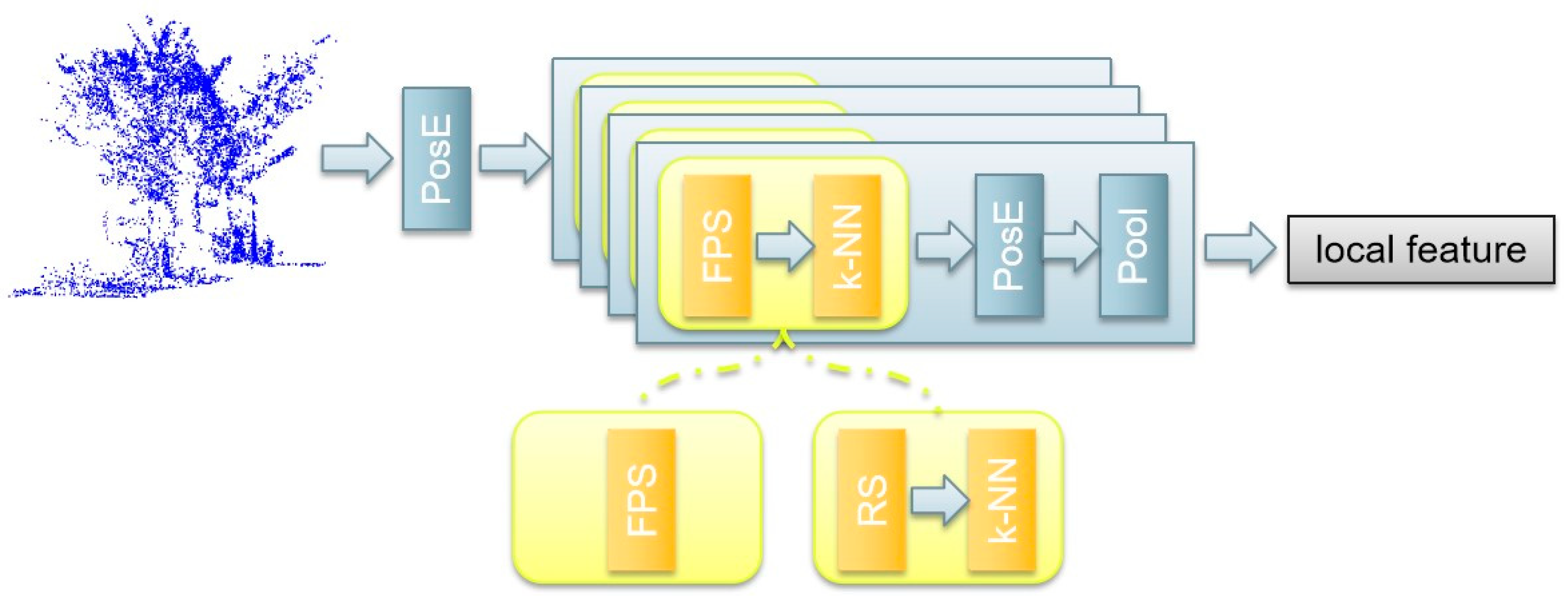
The local feature aggregation (LFA) module combines the positional encoding in the transformer [29] with sampling and grouping strategies, which is shown in Figure 1. The positional encoder (PosE) transforms the raw coordinates of the point cloud into high dimensional vectors to achieve feature embedding without learnable maps. The PosE utilizes the trigonometric function to encode the low feature vector of the point into a high dimensional vector during the inherent nature of trigonometric functions. The PosE can well capture fine-grained structural variations of 3D shapes and well encode relative positional information between different points in point clouds. Taking the encoding feature of point on the axis as an example, the process can be represented by the following formula:
where denotes the encoded feature vector on the axis, denotes the channel index, denotes the dimension of encoded feature vectors, and control the magnitude and wavelengths, respectively. The special process of encoding the point coordinates into a higher dimensional vector is represented by Formula (2).
where denote the encoded vectors on three axes.
The other core of the local feature aggregation module is the set abstraction (SA) module. The iterative SA layer can process the point cloud in each hierarchical level and perform dense prediction by propagating point features along the neighbor region. The SA layer comprises the sampling layer, the positional encoding, and the pooling. The sampling layer is used to find the neighbor points within a local region of each centroid. Different methods can be used to obtain the centroid, including farthest point sampling (FPS) and random sampling (RS). After that, the k-NN is used to group neighbor points among the centroid. The PosE can reveal the local patterns, and the pooling layer utilizes both max and average pooling for local feature aggregation. In each SA layer, we obtain the local aggregated centers, which are fed into the next stage SA layer. Finally, after all 4 stages, a local feature map of the input point cloud is acquired.
2.2. Fusion Segmentation Module
In Figure 2, the fusion segmentation module (Fus-Seg) shows an intuitive synergy [30,31] between different layers in the network. Then, the module generates labels for every point in the point cloud to extend the expression dimensions of the point cloud features.
When inputting a batch of (Layer 1 and Layer 2) pairs, the fusion segmentation (Fus-Seg) module uses segmentation (Seg) blocks to generate the prediction point labels vector (pre-labels) for each point input. The pre-labels vectors of the same point in the input point cloud are represented as and . The segmentation (Seg) block is a learnable operation that is trained by finding the best across pairing in the multi-embedding space [32]. To enhance the interactivity between feature extraction layers in the network, the Fus-Seg module introduces a multi-embedding space by two jointly input layers’ pre-labels, which ensures that all pairings that cross two pre-labels actually occur in the space. The advantage of the multi-embedding space is that it can maximize the cosine similarity of real pairings in the point cloud, and minimize the cosine similarity of incorrect pairings. The size of the multi-embedding space is , and depends on the number of segmentation parts when the network is training. The across pairings in the multi-embedding space are represented as . When , the across pairings are seen as real pairings, and when , they are incorrect pairings.
In addition to increasing the communication of the feature extraction layers in the network, the Fus-Seg module tags points to enrich the features of point clouds. After the multi-embedding space, max pooling is adopted to obtain a label vector for each point. The size of a label vector is , and after max pooling, the size of the label matrix of the point cloud is . Then, the label matrix is fed back to per point features by matrix multiplication, with the features of Layer 2 with each of the point features. The label matrix is regarded as an annotation, which can be used to extend the dimension of the feature map, which is (). Moreover, the label matrix is full of information with segmentation scores, which means the label matrix can be seen as a weight matrix as well. It can be used to sift evaluation factors in the feature maps and enhance the effect of features that play a more important role in the process of network segmentation.
2.3. DFSNet Structure Design
The DFSNet structure is composed of an input layer, a local feature aggregation module, the dynamic segmentation layer, and the output layer. The details of each part are as follows:
Input layer: The input data of the network constitute the point clouds of the orchard scene, which are collective in nature. Each point in point clouds has three column vectors (X, Y, Z), which represent the 3D coordinates. From the perspective of the input data structure, the size of the input point is , where is the number of point clouds and is the feature dimension of each data point. Moreover, considering that the point clouds collected by the LiDAR equipped on the plant protection robot are relatively sparse, the point clouds need to be down-sampled before entering the training phase.
Local feature aggregation (LFA) layer: The LFA module consists of position encoding and 3 stages of SA layers. These SA layers are used to aggregate the features of the point cloud and increase the feature size of each point of each point cloud. In the data of the SA layer, the data size of the point cloud data is reduced to of the original data size after each stage. In the network, the input point cloud number is . After three data SA layers, the size of the point is (). Then, a reconstruction operation that is performed on the point cloud makes the number of point clouds back to . Meanwhile, the feature of the point size is gradually up, and the dimension of the local feature is .
The dynamic segmentation layer: The dynamic segmentation layer includes a Fus-Seg module and an inverted residual block [33]. The Fus-Seg module is used in the network to connect the layers and enhance the expression ability of each point. After the Fus-Seg module, the change in the feature map of the point cloud is (). The inverted residual block that includes three convolutions is used to learn features of the point cloud. The inversion operation allows significant reduction in the memory footprint needed during inference by never fully materializing large intermediate tensors. The block takes as an input a low dimensional compressed representation, which is first expanded to a high dimensional representation; then, the feature is subsequently projected back to a low dimensional representation, that is, ().
Output layer: The output layer of the network is a fully connected layer, the function of which is to map the learned features to the sample label space. The output of the network is the predicted semantics of all points with a size of , where is the number of classes in the dataset. In the simple-scale dataset, . In the complex-scale dataset, .
The specific DFSNet architecture is shown in Figure 3 below.
3. Results
3.1. Dataset Details
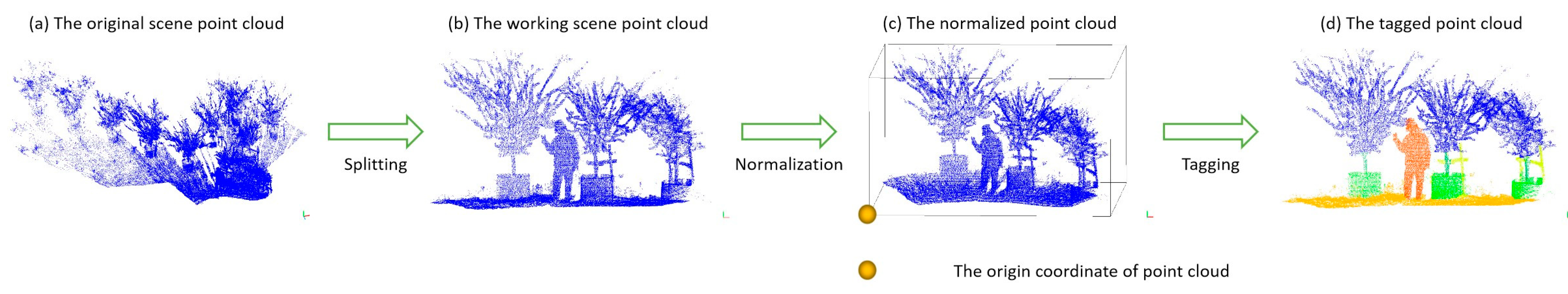
In this study, we used a self-made dataset collected in a real nursery scene. The dataset satisfies the requirements of unstructured forestry scenes, and can be used to measure the performance of the semantic segmentation network. The experimental site selected for this study is a nursery located on 32.12° N. 119.31° E, Zhenjiang, Jiangsu, China. The nursery provides varieties of common landscape orchards and forestry scenes to make the trained models of deep learning networks obtain different application scenes. To ensure sufficient growing space, a distance of 2 to 5 m is maintained between each tree trunk. Moreover, all of the trees are planted in cultivation pots, and some of the trunks are supported by sturdy wooden stakes. To create experimental datasets, we utilized the Livox Horizon scanner to collect the original point clouds. And the CloudCompare (Paris, France) played an important role on subsequent processing of collected point clouds. The software is employed to filter the noise point clouds, split the original scene point cloud after filtering into smaller working scenes, normalize these point clouds of working scenes, and tag segmented point clouds. Figure 4a to Figure 4b show the processing of a splitting of an original scene into a working scene. A typical complete point cloud for a working scene (2–3 trees and other objects in the orchard scene) normally includes 10–60 k points after split processing. For better trained models of network generalization, working scene point clouds need to be normalized on coordinate positions. Considering the perspective of LiDAR when the network is deployed to the orchard robot, we framed the point cloud of working scenes, and set the lower left point of the box as the origin coordinate, then calculated the coordinates of points in the point cloud by translation. An example of a group of normalized point clouds is depicted in Figure 4c. Then, we tagged the point, and the results of a group of scenes are shown in Figure 4d. The format of the dataset files is .txt, and the files include 3D coordinates of point clouds and labels of each point shown as (X, Y, Z, Label).
To obtain a greater quality of point cloud data for network training based on the distinction of work scenes complexity, we further divided the segmentation into two cases: a simple-scale dataset and a complex-scale dataset. The simple-scale dataset contains only trees and grounds. The complex-scale dataset stands for orchard scenes containing more objects, such as people, indicators, and other objects. Examples of the raw and labeled point cloud and semantic segmentation results of the scenes are shown in Figure 5. To realize the 3D point cloud semantic segmentation of the natural orchard scene, the complex-scale dataset and simple-scale dataset are used as the training dataset and test dataset. In the complex-scale dataset, eight semantic labels were applied for the training set, namely, leaves of trees (leaves), trunks of tree (trunks), pots for planting trees (pots), scaffolds for protecting the growth of trees (scaffolds), grounds, people, indicators, and other objects (others). In the program, the corresponding values were set for these eight tags, i.e., 0, 1, 2, 3, 4, 5, 6, and 7. In the simple-scale dataset, five semantic labels were applied for the training set, namely leaves, trunks, pots, scaffolds, and grounds. The corresponding values were set for five tags, i.e., 0, 1, 2, 3, 4, and 5. The trained network can be used to segment tree phenotypes in orchard environments. In addition, the trained model can also detect some obstacles in the orchards. The model plays an important role in the perception system of agricultural robots, and can be used in the autonomous control system and the autonomous navigation of plant protection robots. The complex-scale dataset used 206 of 309 scenes to create the dataset for training, and the rest of the scenes were used to perform training validation and evaluation. And the simple-scale dataset used 360 of 535 scenes to create the dataset for training. Each dataset includes from 30,000 to 60,000 points, and 4096 randomly sampled points in every point cloud as pre-processing before input to the network.
3.2. Experimental Hardware Equipment
The network was developed based on PyTorch-1.13.1. The network training and testing were performed using an NVIDIA RTX-3080Ti (12 GB).
3.3. Training Details
When training a deep learning network, a faster optimizer can improve the efficiency of network training, which reduces the time cost of implementing the same network training, or achieves a smaller error under the same budget. We mainly compared SGD, Adam [34], and AdamW [35] with Sophia [36], which are dominantly used optimizers on deep learning networks. The hyper parameters of optimizers during the network training are shown in Table 2. Figure 6 illustrates the training accuracy curve and loss curve on DFSNet with the same number of hyper parameters. Sophia achieves better accuracy and better stability loss than SGD, Adam, and AdamW. Thus, we used Sophia as the network optimizer during training.
3.4. Semantic Segmentation on Benchmarks
In the field of 3D point cloud semantic segmentation, the and are the two main indicators used to evaluate the effect of semantic segmentation. The is an important indicator for measuring the accuracy of the segmentation. The mainly calculates the ratio between the intersection and union of the two sets. The calculates the according to each class, and then takes the average.
is the real quantity, and is the number of classes (including empty classes). represents the number of predictions for the true value of as , and represents the number of predictions for the true value of as . and represent false positives and false negatives, respectively.
The is the simplest metric calculation, the probability that the semantic annotation result of each sample will be consistent with the actual data annotation type. The accuracy is the ratio between the model’s correct predictions on all test datasets and the overall number.
represents the number of the model’s correct predictions on the test datasets, and represents the overall number of all the test datasets.
3.5. Processing of Network Building
We first analyzed the effect of the number of network layers on segmentation performance. Table 3 shows the training results for the different number layers of the network. The output layer means the number of the dynamic segmentation layer of the network. For example, if the output layer is three, there are three dynamic segmentation layers. When the number of the layer is three, the Acc and mIoU reached their optimal values of this training; the optimal segmentation accuracy is 78.89%, and the mIoU is 73.02%.
Figure 7 is the training result of the tensorboard. Figure 6a shows the relationship between the segmentation accuracy (Acc) and the number of iterations (epoch), and Figure 6b shows the function graph of the relationship between the loss function and the number of iterations (epoch).
It can be seen from the above training log that when the number of epochs is less than 20, the segmentation accuracy already reaches 0.8, and when the number of epochs = 60, the segmentation accuracy reaches 0.95. In addition, the loss function continues to decrease with a continuous increase in training times, and finally remains at approximately 0.05. Compared to the other numbers of layers, the three-layer network is smoother, proving it is steadier.
3.6. Sampling and Grouping Strategy
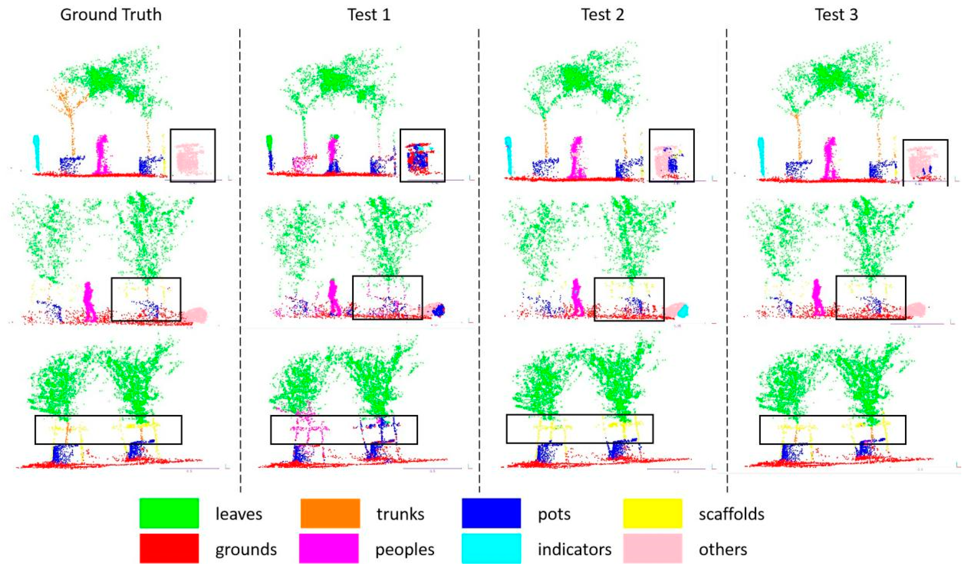
DFSNet applies an iterative farthest point sampling (FPS) or random sampling (RS) strategy to sample () centroids from a point cloud with points, and then uses -nearest neighbor (-NN) to gather points within the neighborhood of each centroid. Table 4 shows the evaluation of segmentation accuracy on centroids sampling and neighbor points grouping strategy by using the complex-scale dataset () on the three-layer DFSNet. Simultaneously, a line graph is plotted in Figure 8 to illustrate the training results of the ablation study in the three strategies, demonstrating the superiority of the sampling layer with FPS and -NN. Test 1 is the model that only uses the FPS sampling layer without the grouping strategy. Experimental results show that grouping strategy is necessary, though the network iterates faster without it. Test 2 and Test 3 compare the sample layer that uses FPS and RS sampling strategies, respectively. The experimental results show that the sample layer with FPS achieves a higher score compared to the layer using RS.
Figure 9 shows the results of the semantic segmentation of the 3D point cloud obtained by these three sampling strategies on the simple-scale and complex-scale datasets. The experiment results show that the semantic tags that the network can segment include leaves of trees, trunks of trees, trees planted in pots, scaffolds, grounds, people, indicators, and others. In the orchard scenes, Test 3 shows the best semantic segmentation effect during these sampling and grouping strategies, and Test 3 has the strongest generalization ability. From the comparison results of the segmentation in black boxes in the figure, Test 3 can clearly segment indicators, people, others, and some details in the orchard field.
3.7. Segmentation in Orchards
This section evaluates the network performance in the simple-scale and complex-scale datasets, and compares it with PointNet, PointNet++, and Point-NN. We first trained the simple-scale and all-scale dataset (combines the simple-scale dataset and the complex-scale dataset) separately by these networks, then tested the networks on different datasets via trained models. According to the quantitative results in Table 5, DFSNet outperforms these typical networks in orchard fields in the segmentation metrics. Among them, when networks both train and test on the simple-scale dataset, the accuracy of DFSNet improves performance by 5.6% over PointNet, and the mIoU improves by 22.32% over PointNet, 1.62% over PointNet++, 1.14% over D-PointNet++, 7.28% over DGCNN, and 25.46% over Point-NN. When the all-scale dataset is used as the training dataset and networks were tested on the simple-scale dataset, we see an 8.19% improvement over PointNet, a 1.12% improvement over PointNet++, a 0.81% improvement over D-PointNet++, and a 1.39% improvement over DGCNN in Acc; then, we also see a 36.58% improvement over PointNet, a 9.27% improvement over PointNet++, a 7.78% improvement over D-PointNet++, a 9.06% improvement over DGCNN, and a 22.12% improvement over Point-NN in mIoU. While testing networks on the complex-scale dataset, the proposed network improves orchard fields segmentation accuracy by 14.14% over PointNet, by 4.96% over PointNet++, by 4.10% over D-PointNet++, and by 3.91% over DGCNN. The network improves mIoU by 22.77% over PointNet, 8.41% over PointNet++, 3.44% over D-PointNet++, 8.49% over DGCNN, and 25.48% over Point-NN. Overall, using networks to segment the scenes on the all-scale dataset, we obtain a 11.73% improvement in Acc and a 28.19% improvement in mIoU when compared to PointNet, a 3.76% improvement in Acc and a 9.89% improvement in mIoU compared to PointNet++, a 2.36% improvement in Acc and a 6.33% improvement in mIoU when compared to D-PointNet++, a 2.74% improvement in Acc and a 9.89% improvement in mIoU over DGCNN, and a 24.69% improvement in mIoU over Point-NN. Figure 10 and Figure 11 show the visualization of the segmentation. As shown in the figures, our DFSNet can accurately segment tree point clouds and recognize objects from the orchard to achieve on par or better segmentation results when compared to PointNet and PointNet++. PointNet produces many false negatives for the points, which is due to the global features without aggregation. PointNet++ has apparent benefits, as compared to PointNet, for segmenting the scenes, but it is still experiences interference by the coordinate values of points, and does not achieve precise edging of different categories. During the experiments, the ability of DFSNet is significantly the best over PointNet, PointNet++, and Point-NN. The improvement in the proposed network may be attributed to the pre-processing local feature aggregation layer and the dynamic segmentation layer, and its ability to better extract point cloud features of orchard environments through DFSNet learning.
4. Conclusions
Orchards play a crucial role in agricultural production. To facilitate the efficient management of orchards and the practical applications of agricultural robots, a sensory perceptual system is necessary. In this research, a 3D point cloud semantic segmentation network called DFSNet for the unstructured orchard fields was proposed, and some good semantic segmentation results were achieved. The proposed network utilized a local feature aggregation (LFA) module and three fusion segmentation (Fus-Seg) modules to improve the training performance when dealing with imbalanced class problems. Meanwhile, the impacts of network depth and 3D point cloud sampling and grouping strategies on the semantic segmentation were compared and analyzed. The test results showed that deeper deep learning neural network is helpful for improving the accuracy of semantic segmentation, and the best sampling strategies we studied use FPS to sample and k-NN as the grouping strategy. The key to semantic segmentation depends on whether the relevant features in the 3D point cloud data can effectively be extracted. The training experimental results show that the best accuracy of 3D point cloud semantic segmentation can reach 89.43%, and the mIoU can reach 74.05% on the datasets that combine the simple-scale dataset and the complex-scale dataset. Comparing DFSNet with the other networks, the accuracy value of the proposed network is 11.73%, 3.76%, 2.36%, and 2.74% higher than the PointNet, PointNet++, D-PointNet++ and DGCNN, respectively. Meanwhile, the mIoU of the proposed network is better by 28.19%, 9.89%, 6.33%, 9.89%, and 24.69% compared with the PointNet, PointNet++, D-PointNet++, DGCNN, and Point-NN, respectively. Both the accuracy and mIoU ensure quality segmentation of the orchard scene.
In practical applications, the proposed DFSNet can provide more accurate information about the orchard scenes such as ground filtering, object identification, tree phenotyping, and other related information. Ground and object detection is the basis for accurate identification of tree row paths, with path planning being the key to orchard management. Additionally, tree phenotype information such as crowns and trunks can be used to realize target locations, which is beneficial to agricultural robots tasks, for example, autonomous variable rate spraying, autonomous fruit picking, and so on. Thus, the proposed network holds practical significance for orchard management. In subsequent studies, we intend to obtain more experimental results via our hardware platform and perception algorithm designed for orchard environments.
Author Contributions
Conceptualization, C.L. and H.L.; methodology, X.B. and Y.S.; software, X.B. and J.X.; validation, C.L., H.L. and G.Y.; formal analysis, Y.S.; investigation, Y.S.; resources, H.L.; data curation, J.X.; writing—original draft preparation, X.B.; writing—review and editing, H.L. and G.Y.; visualization, X.B.; supervision, H.L.; project administration, Y.S.; funding acquisition, H.L. All authors have read and agreed to the published version of the manuscript.
Funding
This research was funded by the National Natural Science Foundation of China under grant project no. 32171908.
Institutional Review Board Statement
Not applicable.
Informed Consent Statement
Not applicable.
Data Availability Statement
Data will be made available upon request.
Conflicts of Interest
The authors declare no conflicts of interest.
References
- Liu, F.; Wang, H.; Li, L.; Xuan, J. Status quo, problems and development countermeasures of China’s facility fruit tree industry. China Fruit Tree 2021, 217, 1–4. [Google Scholar]
- Abramczyk, B.; Pecio, Ł.; Kozachok, S.; Kowalczyk, M.; Marzec-Grządziel, A.; Król, E.; Gałązka, A.; Oleszek, W. Pioneering Metabolomic Studies on Diaporthe eres Species Complex from Fruit Trees in the South-Eastern Poland. Molecules 2023, 28, 1175. [Google Scholar] [CrossRef] [PubMed]
- Sayyad-Amin, P. A review on breeding fruit trees against climate changes. Erwerbs-Obstbau 2022, 64, 697–701. [Google Scholar] [CrossRef]
- Gao, Y.; Tian, G.; Gu, B.; Zhao, J.; Liu, Q.; Qiu, C.; Xue, J. A Study on the Rapid Detection of Steering Markers in Orchard Management Robots Based on Improved YOLOv7. Electronics 2023, 12, 3614. [Google Scholar] [CrossRef]
- Raikwar, S.; Fehrmann, J.; Herlitzius, T. Navigation and control development for a four-wheel-steered mobile orchard robot using model-based design. Comput. Electron. Agric. 2022, 202, 107410. [Google Scholar] [CrossRef]
- Wang, X.; Kang, H.; Zhou, H.; Au, W.; Chen, C. Geometry-aware fruit grasping estimation for robotic harvesting in apple orchards. Comput. Electron. Agric. 2022, 193, 106716. [Google Scholar] [CrossRef]
- Chen, Y.; Xiong, Y.; Zhang, B.; Zhou, J.; Zhang, Q. 3D point cloud semantic segmentation toward large-scale unstructured agricultural scene classification. Comput. Electron. Agric. 2021, 190, 106445. [Google Scholar] [CrossRef]
- Kang, H.; Wang, X. Semantic segmentation of fruits on multi-sensor fused data in natural orchards. Comput. Electron. Agric. 2023, 204, 107569. [Google Scholar] [CrossRef]
- Wang, Y.; Yang, C.; Hu, M.; Zhang, J.; Li, Q.; Zhai, G.; Zhang, X.-P. Identification of deep breath while moving forward based on multiple body regions and graph signal analysis. In Proceedings of the ICASSP 2021—2021 IEEE International Conference on Acoustics, Speech and Signal Processing (ICASSP), Toronto, ON, Canada, 6–11 June 2021; pp. 7958–7962. [Google Scholar]
- Zeng, L.; Feng, J.; He, L. Semantic segmentation of sparse 3D point cloud based on geometrical features for trellis-structured apple orchard. Biosyst. Eng. 2020, 196, 46–55. [Google Scholar] [CrossRef]
- Wang, D.; He, D. Fusion of Mask RCNN and attention mechanism for instance segmentation of apples under complex background. Comput. Electron. Agric. 2022, 196, 106864. [Google Scholar] [CrossRef]
- Turgut, K.; Dutagaci, H.; Rousseau, D. RoseSegNet: An attention-based deep learning architecture for organ segmentation of plants. Biosyst. Eng. 2022, 221, 138–153. [Google Scholar] [CrossRef]
- Jin, S.; Sun, X.; Wu, F.; Su, Y.; Li, Y.; Song, S.; Xu, K.; Ma, Q.; Baret, F.; Jiang, D.; et al. Lidar sheds new light on plant phenomics for plant breeding and management: Recent advances and future prospects. ISPRS J. Photogramm. Remote. Sens. 2021, 171, 202–223. [Google Scholar] [CrossRef]
- Li, Y.; Wen, W.; Miao, T.; Wu, S.; Yu, Z.; Wang, X.; Guo, X.; Zhao, C. Automatic organ-level point cloud segmentation of maize shoots by integrating high-throughput data acquisition and deep learning. Comput. Electron. Agric. 2022, 193, 106702. [Google Scholar] [CrossRef]
- Qi, C.R.; Yi, L.; Su, H.; Guibas, L.J. Pointnet++: Deep hierarchical feature learning on point sets in a metric space. In Proceedings of the NIPS’17: Proceedings of the 31st International Conference on Neural Information Processing Systems, Long Beach, CA, USA, 6–9 December 2017; Volume 30. [Google Scholar]
- Xu, J.; Liu, H.; Shen, Y.; Zeng, X.; Zheng, X. Individual nursery trees classification and segmentation using a point cloud-based neural network with dense connection pattern. Sci. Hortic. 2024, 328, 112945. [Google Scholar] [CrossRef]
- Zhao, H.; Jiang, L.; Fu, C.-W.; Jia, J. Pointweb: Enhancing local neighborhood features for point cloud processing. In Proceedings of the 2019 IEEE/CVF Conference on Computer Vision and Pattern Recognition (CVPR), Long Beach, CA, USA, 15–20 June 2019; pp. 5565–5573. [Google Scholar]
- Duan, Y.; Zheng, Y.; Lu, J.; Zhou, J.; Tian, Q. Structural relational reasoning of point clouds. In Proceedings of the 2019 IEEE/CVF Conference on Computer Vision and Pattern Recognition (CVPR), Long Beach, CA, USA, 15–20 June 2019; pp. 949–958. [Google Scholar]
- Ma, X.; Qin, C.; You, H.; Ran, H.; Fu, Y. Rethinking network design and local geometry in point cloud: A simple residual MLP framework. arXiv 2022, arXiv:2202.07123. [Google Scholar]
- Wang, Y.; Sun, Y.; Liu, Z.; Sarma, S.E.; Bronstein, M.M.; Solomon, J.M. Dynamic graph CNN for learning on point clouds. ACM Trans. Graphic. 2019, 38, 1–12. [Google Scholar] [CrossRef]
- Landrieu, L.; Simonovsky, M. Large-scale point cloud semantic segmentation with superpoint graphs. In Proceedings of the 2018 IEEE/CVF Conference on Computer Vision and Pattern Recognition, Salt Lake City, UT, USA, 18–23 June 2018; pp. 4558–4567. [Google Scholar]
- Te, G.; Hu, W.; Zheng, A.; Guo, Z. Rgcnn: Regularized graph cnn for point cloud segmentation. In Proceedings of the 26th ACM International Conference on Multimedia, Seoul, Republic of Korea, 22–26 October 2018; pp. 746–754. [Google Scholar]
- Qi, C.R.; Su, H.; Mo, K.; Guibas, L.J. Pointnet: Deep learning on point sets for 3d classification and segmentation. In Proceedings of the 2017 IEEE Conference on Computer Vision and Pattern Recognition (CVPR), Honolulu, HI, USA, 21–26 July 2017; pp. 652–660. [Google Scholar]
- Dosovitskiy, A.; Beyer, L.; Kolesnikov, A.; Weissenborn, D.; Zhai, X.; Unterthiner, T.; Dehghani, M.; Minderer, M.; Heigold, G.; Gelly, S.; et al. An image is worth 16x16 words: Transformers for image recognition at scale. arXiv 2020, arXiv:2010.11929. [Google Scholar]
- Liu, Z.; Lin, Y.; Cao, Y.; Hu, H.; Wei, Y.; Zhang, Z.; Lin, S.; Guo, B. Swin transformer: Hierarchical vision transformer using shifted windows. In Proceedings of the 2021 IEEE/CVF International Conference on Computer Vision (ICCV), Montreal, QC, Canada, 10–17 October 2021; pp. 10012–10022. [Google Scholar]
- Touvron, H.; Cord, M.; Douze, M.; Massa, F.; Sablayrolles, A.; Jégou, H. Training data-efficient image transformers & distillation through attention. In Proceedings of the 38th International Conference on Machine Learning, Virtual, 18–24 July 2021; pp. 10347–10357. Available online: http://proceedings.mlr.press/v139/touvron21a/touvron21a.pdf (accessed on 29 March 2024).
- Rao, Y.; Zhao, W.; Tang, Y.; Zhou, J.; Lim, S.N.; Lu, J. Hornet: Efficient high-order spatial interactions with recursive gated convolutions. arXiv 2022, arXiv:2207.14284. [Google Scholar]
- Zhang, R.; Wang, L.; Guo, Z.; Wang, Y.; Gao, P.; Li, H.; Shi, J. Parameter is Not All You Need: Starting from Non-Parametric Networks for 3D Point Cloud Analysis. arXiv 2023, arXiv:2303.08134. [Google Scholar]
- Vaswani, A.; Shazeer, N.; Parmar, N.; Uszkoreit, J.; Jones, L.; Gomez, A.N.; Kaiser, Ł.; Polosukhin, I. Attention is all you need. In Proceedings of the 31st Conference on Neural Information Processing Systems (NIPS 2017), Long Beach, CA, USA, 4–9 December 2017; Volume 30. [Google Scholar]
- Chowdhury, P.N.; Bhunia, A.K.; Sain, A.; Koley, S.; Xiang, T.; Song, Y.Z. What Can Human Sketches Do for Object Detection? In Proceedings of the 2023 IEEE/CVF Conference on Computer Vision and Pattern Recognition (CVPR), Vancouver, BC, Canada, 17–24 June 2023; pp. 15083–15094. [Google Scholar]
- Jiang, B.; He, J.; Yang, S.; Fu, H.; Li, T.; Song, H.; He, D. Fusion of machine vision technology and AlexNet-CNNs deep learning network for the detection of postharvest apple pesticide residues. Artif. Intell. Agric. 2019, 1, 1–8. [Google Scholar] [CrossRef]
- Radford, A.; Kim, J.W.; Hallacy, C.; Ramesh, A.; Goh, G.; Agarwal, S.; Sastry, G.; Askell, A.; Mishkin, P.; Clark, J.; et al. Learning transferable visual models from natural language supervision. In Proceedings of the 38th International Conference on Machine Learning, Virtual, 18–24 July 2021; pp. 8748–8763. Available online: http://proceedings.mlr.press/v139/radford21a/radford21a.pdf (accessed on 29 March 2024).
- Sandler, M.; Howard, A.; Zhu, M.; Zhmoginov, A.; Chen, L. Mobilenetv2: Inverted residuals and linear bottlenecks. In Proceedings of the 2018 IEEE/CVF Conference on Computer Vision and Pattern Recognition, Salt Lake City, UT, USA, 18–23 June 2018; pp. 4510–4520. [Google Scholar]
- Kingma, D.P.; Ba, J. Adam: A method for stochastic optimization. arXiv 2014, arXiv:1412.6980. [Google Scholar]
- Loshchilov, I.; Hutter, F. Decoupled weight decay regularization. arXiv 2017, arXiv:1711.05101. [Google Scholar]
- Liu, H.; Li, Z.; Hall, D.; Liang, P.; Ma, T. Sophia: A Scalable Stochastic Second-order Optimizer for Language Model Pre-training. arXiv 2023, arXiv:2305.14342. [Google Scholar]
Figure 1.
The local feature aggregation (LFA) module. Yellow blocks indicate the sampling and grouping strategies. PosE: positional encoder, FPS: farthest point sampling, RS: random sampling, k-NN: k-nearest neighbor grouping, Pool: max pooling. An SA (set abstraction) module includes a sampling and grouping strategies block, a PosE, and a Pool, and there are 4 stages of SA modules in the LFA.

Figure 2.
Fusion segmentation module (Fus-Seg). While standard convolution jointly trains point cloud feature segmentation (Seg) to predict point labels, the multi-model embedding space jointly trains two layers’ segmentation to predict the correct pairings of a batch of (Layer 1 and Layer 2) training examples. : the pre-labels of one point in a point cloud are obtained by Layer 1 Seg; : the pre-labels of the same point are obtained by Layer 2 Seg. : feature map size of input point clouds; : the feature map size of output point clouds; : the segmentation number of DFSNet.

Figure 3.
The structure of DFSNet. LFA, local feature aggregation layer; Fus-Seg, fusion segmentation modules; MLP, shared multi-layer perceptron.
Figure 3.
The structure of DFSNet. LFA, local feature aggregation layer; Fus-Seg, fusion segmentation modules; MLP, shared multi-layer perceptron.

Figure 4.
The visualization of point cloud data processing. (a) The original scene point cloud, which is filtered from the collected point cloud. (b) The working scene point cloud, which is split from the original scene point cloud. (c) Normalize the coordinates of each set of point clouds. (d) Segment different parts of the point clouds of the scene and represent them in different colors for labels of the segmentation results.

Figure 5.
The raw point clouds and their segmentation results; different colors represent different labels of segmentation. (a,b) represent the complex-scale segmentation. (c,d) represent the simple-scale segmentation.
Figure 5.
The raw point clouds and their segmentation results; different colors represent different labels of segmentation. (a,b) represent the complex-scale segmentation. (c,d) represent the simple-scale segmentation.

Figure 6.
(a) The training accuracies and training epochs and (b) the loss functions and training epochs.
Figure 6.
(a) The training accuracies and training epochs and (b) the loss functions and training epochs.

Figure 7.
Function graphs of the relationships between (a) the training accuracy and the training epoch and (b) the loss function and training epoch.
Figure 7.
Function graphs of the relationships between (a) the training accuracy and the training epoch and (b) the loss function and training epoch.

Figure 8.
Function graphs of the relationships between (a) the training accuracy and the training epochs and (b) the loss function and training epochs.
Figure 8.
Function graphs of the relationships between (a) the training accuracy and the training epochs and (b) the loss function and training epochs.

Figure 9.
Complete semantic segmentation using the different sampling strategies. Different colors correspond to different segmentation labels. The black boxes mark the segmentation error parts in the point cloud.
Figure 9.
Complete semantic segmentation using the different sampling strategies. Different colors correspond to different segmentation labels. The black boxes mark the segmentation error parts in the point cloud.

Figure 10.
Semantic segmentation results of different networks in the simple-scale dataset. The black boxes mark the segmentation error parts in the point cloud.
Figure 10.
Semantic segmentation results of different networks in the simple-scale dataset. The black boxes mark the segmentation error parts in the point cloud.

Figure 11.
Semantic segmentation results of different networks in the complex-scale dataset. The black boxes mark the segmentation error parts in the point cloud.
Figure 11.
Semantic segmentation results of different networks in the complex-scale dataset. The black boxes mark the segmentation error parts in the point cloud.


Table 1.
Systematic comparison among some representative methods.
| Network | Sampling + Grouping Strategy | Principal Operator | Basic Architecture |
|---|---|---|---|
| PointNet | - | MLP 3 | Branch |
| DGCNN | k-NN 1 | EdgeConv | Branch and Dynamic |
| PointMLP | Geometric affine module | MLP | ResNet |
| PointNet++ | FPS 2 + Region grouping | PointNet layer | U-Net and Hierarchical |
| D-PointNet++ | FPS + Region grouping | Dense PointNet layer | DenseNet and PointNet++ |
| HorNet | - | gnConv 4 | HorBlock and FFN 5 |
1 k-NN: k-nearest neighbor; 2 FPS: farthest point sampling; 3 MLP: multi-layer perceptron; 4 gnConv: recursive gated convolution; 5 FFN: feed-forward network.
Table 2.
Hyper parameters of optimizers during the DFSNet training.
| Hyper Parameters | Value |
|---|---|
| lr 1 | 0.001 |
| betas | (0.9, 0.999) |
| epc 2 | 1 × 10⁻⁸ |
| weight_decay | 1 × 10⁻⁴ |
| Epoch | 150 |
1 lr: learning rate; 2 epc: error of floating-point calculation.
Table 3.
Comparison of layers on network performance.
| Output Layer | Acc (%) | mIoU (%) | Iterate Speed (ms/pc *) |
|---|---|---|---|
| 1 | 72.16 | 62.28 | 13.79 ms |
| 2 | 72.18 | 63.13 | 13.88 ms |
| 3 | 78.89 | 73.02 | 14.08 ms |
* pc: point cloud.
Table 4.
Comparison of sampling and grouping strategies on network performance.
| Test | Sampling + Grouping Strategy | Acc(%) | mIoU(%) | Iterate Speed |
|---|---|---|---|---|
| 1 | FPS 1 | 37.20 | 32.17 | 4.76 ms |
| 2 | RS 2 + k-NN 3 | 75.64 | 66.70 | 17.38 ms |
| 3 | FPS + k-NN | 76.57 | 69.16 | 13.98 ms |
1 FPS: farthest point sampling; 2 RS: random sampling; 3 k-NN: k-nearest neighbor.
Table 5.
Results on semantic segmentation in orchard fields.
| Train Dataset | Test Dataset | Network | Acc (%) | mIoU (%) |
|---|---|---|---|---|
| Simple-scale | Simple-scale | PointNet | 92.02 | 63.08 |
| PointNet++ | 97.24 | 83.78 | ||
| D-PointNet++ | 97.27 | 84.26 | ||
| DGCNN | 95.96 | 78.12 | ||
| Point-NN | - | 59.94 | ||
| Ours | 97.62 | 85.40 | ||
| All-scale (Simple-scale + Complex-scale) | Simple-scale | PointNet | 89.03 | 49.71 |
| PointNet++ | 96.10 | 77.02 | ||
| D-PointNet++ | 96.41 | 78.51 | ||
| DGCNN | 95.83 | 77.23 | ||
| Point-NN | - | 64.17 | ||
| Ours | 97.22 | 86.29 | ||
| Complex-scale | PointNet | 71.69 | 43.95 | |
| PointNet++ | 80.87 | 58.31 | ||
| D-PointNet++ | 81.73 | 63.28 | ||
| DGCNN | 81.92 | 58.23 | ||
| Point-NN | - | 41.24 | ||
| Ours | 85.83 | 66.72 | ||
| All-scale (Simple-scale + Complex-scale) | PointNet | 77.70 | 45.86 | |
| PointNet++ | 85.67 | 64.16 | ||
| D-PointNet++ | 87.07 | 67.72 | ||
| DGCNN | 86.69 | 64.16 | ||
| Point-NN | - | 49.36 | ||
| Ours | 89.43 | 74.05 |
Disclaimer/Publisher’s Note: The statements, opinions and data contained in all publications are solely those of the individual author(s) and contributor(s) and not of MDPI and/or the editor(s). MDPI and/or the editor(s) disclaim responsibility for any injury to people or property resulting from any ideas, methods, instructions or products referred to in the content. |
© 2024 by the authors. Licensee MDPI, Basel, Switzerland. This article is an open access article distributed under the terms and conditions of the Creative Commons Attribution (CC BY) license (https://creativecommons.org/licenses/by/4.0/).
Share and Cite
MDPI and ACS Style
Bu, X.; Liu, C.; Liu, H.; Yang, G.; Shen, Y.; Xu, J. DFSNet: A 3D Point Cloud Segmentation Network toward Trees Detection in an Orchard Scene. Sensors 2024, 24, 2244. https://doi.org/10.3390/s24072244
AMA Style
Bu X, Liu C, Liu H, Yang G, Shen Y, Xu J. DFSNet: A 3D Point Cloud Segmentation Network toward Trees Detection in an Orchard Scene. Sensors. 2024; 24(7):2244. https://doi.org/10.3390/s24072244
Chicago/Turabian StyleBu, Xinrong, Chao Liu, Hui Liu, Guanxue Yang, Yue Shen, and Jie Xu. 2024. "DFSNet: A 3D Point Cloud Segmentation Network toward Trees Detection in an Orchard Scene" Sensors 24, no. 7: 2244. https://doi.org/10.3390/s24072244
Note that from the first issue of 2016, this journal uses article numbers instead of page numbers. See further details here.